

Preliminary Study on Integrated Simulation
289
[19] model. Chen Guangjin and Guo Tianmin proposed a prediction model completely
different from the Vdw-P model. The model was not only simplified in the calculation,
but also greatly improved in the prediction accuracy compared with the traditional model.
Klauda and Sandler [20] introduced Kihara potential model parameters and second virial
coefficients in the process of calculating the fugacity of gas components. Method of
quantum mechanics was also incorporated into this model. The results showed that this
method was more accurate in calculation and has a wider temperature range.
2 Hydraulic and Thermal Calculation of Gas Gathering Pipeline
Network
2.1 Hydraulic Calculation
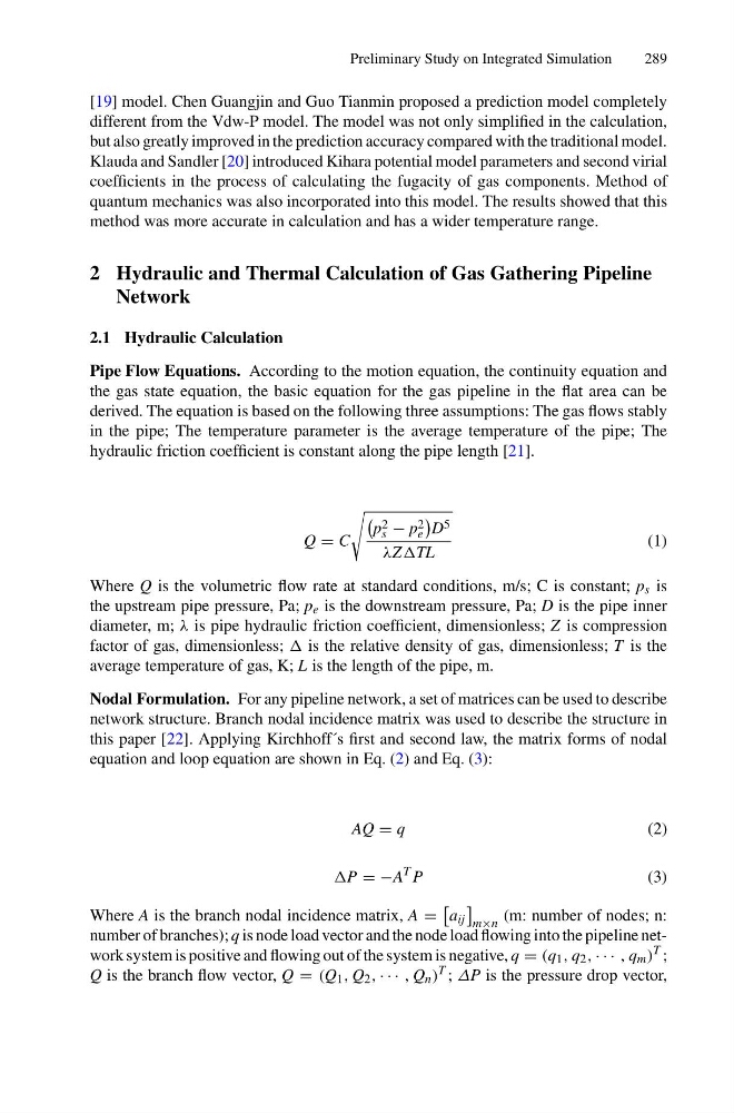
Pipe Flow Equations. According to the motion equation, the continuity equation and
the gas state equation, the basic equation for the gas pipeline in the flat area can be
derived. The equation is based on the following three assumptions: The gas flows stably
in the pipe; The temperature parameter is the average temperature of the pipe; The
hydraulic friction coefficient is constant along the pipe length [21].
Q = C
p 2
s − p 2
e
D 5
λZTL
(1)
Where Q is the volumetric flow rate at standard conditions, m/s; C is constant; p s is
the upstream pipe pressure, Pa; p e is the downstream pressure, Pa; D is the pipe inner
diameter, m; λ is pipe hydraulic friction coefficient, dimensionless; Z is compression
factor of gas, dimensionless; is the relative density of gas, dimensionless; T is the
average temperature of gas, K; L is the length of the pipe, m.
Nodal Formulation. For any pipeline network, a set of matrices can be used to describe
network structure. Branch nodal incidence matrix was used to describe the structure in
this paper [22]. Applying Kirchhoff´s first and second law, the matrix forms of nodal
equation and loop equation are shown in Eq. (2) and Eq. (3):
AQ = q
(2)
P = −A
T P
(3)
Where A is the branch nodal incidence matrix, A =
a ij
m×n
(m: number of nodes; n:
number of branches); q is node load vector and the node load flowing into the pipeline network system is positive and flowing out of the system is negative, q = (q 1 , q 2 , · · · , q m )
T ;
Q is the branch flow vector, Q = (Q 1 , Q 2 , · · · , Q n )
T ; ΔP is the pressure drop vector,
289
[19] model. Chen Guangjin and Guo Tianmin proposed a prediction model completely
different from the Vdw-P model. The model was not only simplified in the calculation,
but also greatly improved in the prediction accuracy compared with the traditional model.
Klauda and Sandler [20] introduced Kihara potential model parameters and second virial
coefficients in the process of calculating the fugacity of gas components. Method of
quantum mechanics was also incorporated into this model. The results showed that this
method was more accurate in calculation and has a wider temperature range.
2 Hydraulic and Thermal Calculation of Gas Gathering Pipeline
Network
2.1 Hydraulic Calculation
Pipe Flow Equations. According to the motion equation, the continuity equation and
the gas state equation, the basic equation for the gas pipeline in the flat area can be
derived. The equation is based on the following three assumptions: The gas flows stably
in the pipe; The temperature parameter is the average temperature of the pipe; The
hydraulic friction coefficient is constant along the pipe length [21].
Q = C
p 2
s − p 2
e
D 5
λZTL
(1)
Where Q is the volumetric flow rate at standard conditions, m/s; C is constant; p s is
the upstream pipe pressure, Pa; p e is the downstream pressure, Pa; D is the pipe inner
diameter, m; λ is pipe hydraulic friction coefficient, dimensionless; Z is compression
factor of gas, dimensionless; is the relative density of gas, dimensionless; T is the
average temperature of gas, K; L is the length of the pipe, m.
Nodal Formulation. For any pipeline network, a set of matrices can be used to describe
network structure. Branch nodal incidence matrix was used to describe the structure in
this paper [22]. Applying Kirchhoff´s first and second law, the matrix forms of nodal
equation and loop equation are shown in Eq. (2) and Eq. (3):
AQ = q
(2)
P = −A
T P
(3)
Where A is the branch nodal incidence matrix, A =
a ij
m×n
(m: number of nodes; n:
number of branches); q is node load vector and the node load flowing into the pipeline network system is positive and flowing out of the system is negative, q = (q 1 , q 2 , · · · , q m )
T ;
Q is the branch flow vector, Q = (Q 1 , Q 2 , · · · , Q n )
T ; ΔP is the pressure drop vector,