

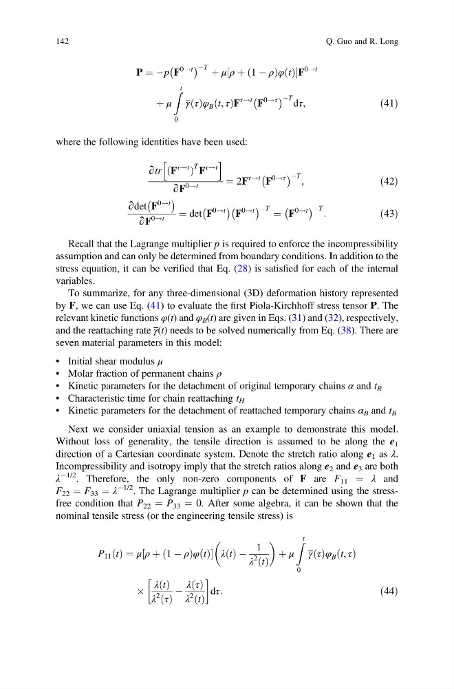
P ¼ Àp F
0!t
À
Á ÀT þ μ ρ þ 1 À ρ
ð
Þφ t
ð Þ
½
F
0!t
þ μ
Z t
0
γ τ
ð Þφ B t, τ
ð ÞF
τ!t F
0!τ
À
Á ÀT dτ,
ð41Þ
where the following identities have been used:
∂tr F
τ!t
ð
Þ
T F
τ!t
h
i
∂F
0!t
¼ 2F
τ!t F
0!τ
À
Á ÀT ,
ð42Þ
∂det F
0!t
À
Á
∂F
0!t
¼ det F
0!t
À
Á
F
0!t
À
Á ÀT ¼ F
0!t
À
Á ÀT :
ð43Þ
Recall that the Lagrange multiplier p is required to enforce the incompressibility
assumption and can only be determined from boundary conditions. In addition to the
stress equation, it can be verified that Eq. (28) is satisfied for each of the internal
variables.
To summarize, for any three-dimensional (3D) deformation history represented
by F, we can use Eq. (41) to evaluate the first Piola-Kirchhoff stress tensor P. The
relevant kinetic functions φ(t) and φ B (t) are given in Eqs. (31) and (32), respectively,
and the reattaching rate γ(t) needs to be solved numerically from Eq. (38). There are
seven material parameters in this model:
• Initial shear modulus μ
• Molar fraction of permanent chains ρ
• Kinetic parameters for the detachment of original temporary chains α and t R
• Characteristic time for chain reattaching t H
• Kinetic parameters for the detachment of reattached temporary chains α B and t B
Next we consider uniaxial tension as an example to demonstrate this model.
Without loss of generality, the tensile direction is assumed to be along the e 1
direction of a Cartesian coordinate system. Denote the stretch ratio along e 1 as λ.
Incompressibility and isotropy imply that the stretch ratios along e 2 and e 3 are both
λ
À1/2
. Therefore, the only non-zero components of F are F 11 ¼ λ and
F 22 ¼ F 33 ¼ λ
À1/2 . The Lagrange multiplier p can be determined using the stressfree condition that P 22 ¼ P 33 ¼ 0. After some algebra, it can be shown that the
nominal tensile stress (or the engineering tensile stress) is
P 11 t
ð Þ ¼ μ ρ þ 1 À ρ
ð
Þφ t
ð Þ
½
λ t
ð Þ À
1
λ
2 t
ð Þ
þ μ
Z t
0
γ τ
ð Þφ B t, τ
ð Þ
Â
λ t
ð Þ
λ
2
τ
ð Þ
À
λ τ
ð Þ
λ
2 t
ð Þ
!
dτ:
ð44Þ
142
Q. Guo and R. Long
0!t
À
Á ÀT þ μ ρ þ 1 À ρ
ð
Þφ t
ð Þ
½
F
0!t
þ μ
Z t
0
γ τ
ð Þφ B t, τ
ð ÞF
τ!t F
0!τ
À
Á ÀT dτ,
ð41Þ
where the following identities have been used:
∂tr F
τ!t
ð
Þ
T F
τ!t
h
i
∂F
0!t
¼ 2F
τ!t F
0!τ
À
Á ÀT ,
ð42Þ
∂det F
0!t
À
Á
∂F
0!t
¼ det F
0!t
À
Á
F
0!t
À
Á ÀT ¼ F
0!t
À
Á ÀT :
ð43Þ
Recall that the Lagrange multiplier p is required to enforce the incompressibility
assumption and can only be determined from boundary conditions. In addition to the
stress equation, it can be verified that Eq. (28) is satisfied for each of the internal
variables.
To summarize, for any three-dimensional (3D) deformation history represented
by F, we can use Eq. (41) to evaluate the first Piola-Kirchhoff stress tensor P. The
relevant kinetic functions φ(t) and φ B (t) are given in Eqs. (31) and (32), respectively,
and the reattaching rate γ(t) needs to be solved numerically from Eq. (38). There are
seven material parameters in this model:
• Initial shear modulus μ
• Molar fraction of permanent chains ρ
• Kinetic parameters for the detachment of original temporary chains α and t R
• Characteristic time for chain reattaching t H
• Kinetic parameters for the detachment of reattached temporary chains α B and t B
Next we consider uniaxial tension as an example to demonstrate this model.
Without loss of generality, the tensile direction is assumed to be along the e 1
direction of a Cartesian coordinate system. Denote the stretch ratio along e 1 as λ.
Incompressibility and isotropy imply that the stretch ratios along e 2 and e 3 are both
λ
À1/2
. Therefore, the only non-zero components of F are F 11 ¼ λ and
F 22 ¼ F 33 ¼ λ
À1/2 . The Lagrange multiplier p can be determined using the stressfree condition that P 22 ¼ P 33 ¼ 0. After some algebra, it can be shown that the
nominal tensile stress (or the engineering tensile stress) is
P 11 t
ð Þ ¼ μ ρ þ 1 À ρ
ð
Þφ t
ð Þ
½
λ t
ð Þ À
1
λ
2 t
ð Þ
þ μ
Z t
0
γ τ
ð Þφ B t, τ
ð Þ
Â
λ t
ð Þ
λ
2
τ
ð Þ
À
λ τ
ð Þ
λ
2 t
ð Þ
!
dτ:
ð44Þ
142
Q. Guo and R. Long