

2 Continuum Mechanics and Thermodynamics of Solids
2.1 Kinematics
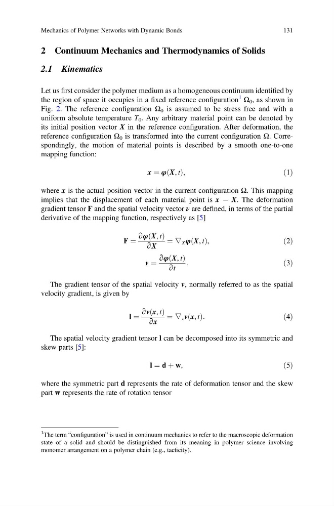
Let us first consider the polymer medium as a homogeneous continuum identified by
the region of space it occupies in a fixed reference configuration
1
Ω 0 , as shown in
Fig. 2. The reference configuration Ω 0 is assumed to be stress free and with a
uniform absolute temperature T 0 . Any arbitrary material point can be denoted by
its initial position vector X in the reference configuration. After deformation, the
reference configuration Ω 0 is transformed into the current configuration Ω. Correspondingly, the motion of material points is described by a smooth one-to-one
mapping function:
x ¼ φ X, t
ð Þ,
ð1Þ
where x is the actual position vector in the current configuration Ω. This mapping
implies that the displacement of each material point is x À X. The deformation
gradient tensor F and the spatial velocity vector ν are defined, in terms of the partial
derivative of the mapping function, respectively as [5]
F ¼
∂φ X, t
ð Þ
∂X
¼ ∇ X φ X, t
ð Þ,
ð2Þ
v ¼
∂φ X, t
ð Þ
∂t
:
ð3Þ
The gradient tensor of the spatial velocity v, normally referred to as the spatial
velocity gradient, is given by
l ¼
∂v x, t
ð Þ
∂x
¼ ∇ x v x, t
ð Þ:
ð4Þ
The spatial velocity gradient tensor l can be decomposed into its symmetric and
skew parts [5]:
l ¼ d þ w,
ð5Þ
where the symmetric part d represents the rate of deformation tensor and the skew
part w represents the rate of rotation tensor
1 The term “configuration” is used in continuum mechanics to refer to the macroscopic deformation
state of a solid and should be distinguished from its meaning in polymer science involving
monomer arrangement on a polymer chain (e.g., tacticity).
Mechanics of Polymer Networks with Dynamic Bonds
131
2.1 Kinematics
Let us first consider the polymer medium as a homogeneous continuum identified by
the region of space it occupies in a fixed reference configuration
1
Ω 0 , as shown in
Fig. 2. The reference configuration Ω 0 is assumed to be stress free and with a
uniform absolute temperature T 0 . Any arbitrary material point can be denoted by
its initial position vector X in the reference configuration. After deformation, the
reference configuration Ω 0 is transformed into the current configuration Ω. Correspondingly, the motion of material points is described by a smooth one-to-one
mapping function:
x ¼ φ X, t
ð Þ,
ð1Þ
where x is the actual position vector in the current configuration Ω. This mapping
implies that the displacement of each material point is x À X. The deformation
gradient tensor F and the spatial velocity vector ν are defined, in terms of the partial
derivative of the mapping function, respectively as [5]
F ¼
∂φ X, t
ð Þ
∂X
¼ ∇ X φ X, t
ð Þ,
ð2Þ
v ¼
∂φ X, t
ð Þ
∂t
:
ð3Þ
The gradient tensor of the spatial velocity v, normally referred to as the spatial
velocity gradient, is given by
l ¼
∂v x, t
ð Þ
∂x
¼ ∇ x v x, t
ð Þ:
ð4Þ
The spatial velocity gradient tensor l can be decomposed into its symmetric and
skew parts [5]:
l ¼ d þ w,
ð5Þ
where the symmetric part d represents the rate of deformation tensor and the skew
part w represents the rate of rotation tensor
1 The term “configuration” is used in continuum mechanics to refer to the macroscopic deformation
state of a solid and should be distinguished from its meaning in polymer science involving
monomer arrangement on a polymer chain (e.g., tacticity).
Mechanics of Polymer Networks with Dynamic Bonds
131