

length ‘(t). These data are converted, using the average length h‘(t)i to extensions
δ‘(t), which form the raw input to the correlator ϕ(t) in Eq. (55), and the subsequent
analysis. To permit the Kramers-Kronig integration across the entire frequency
domain, the high-frequency part of h|δ‘ ω |
2
i is analytically extended.
4.2.1 Simulation Results
First, we investigate the relation between the reversible potential strength ε 0 and the
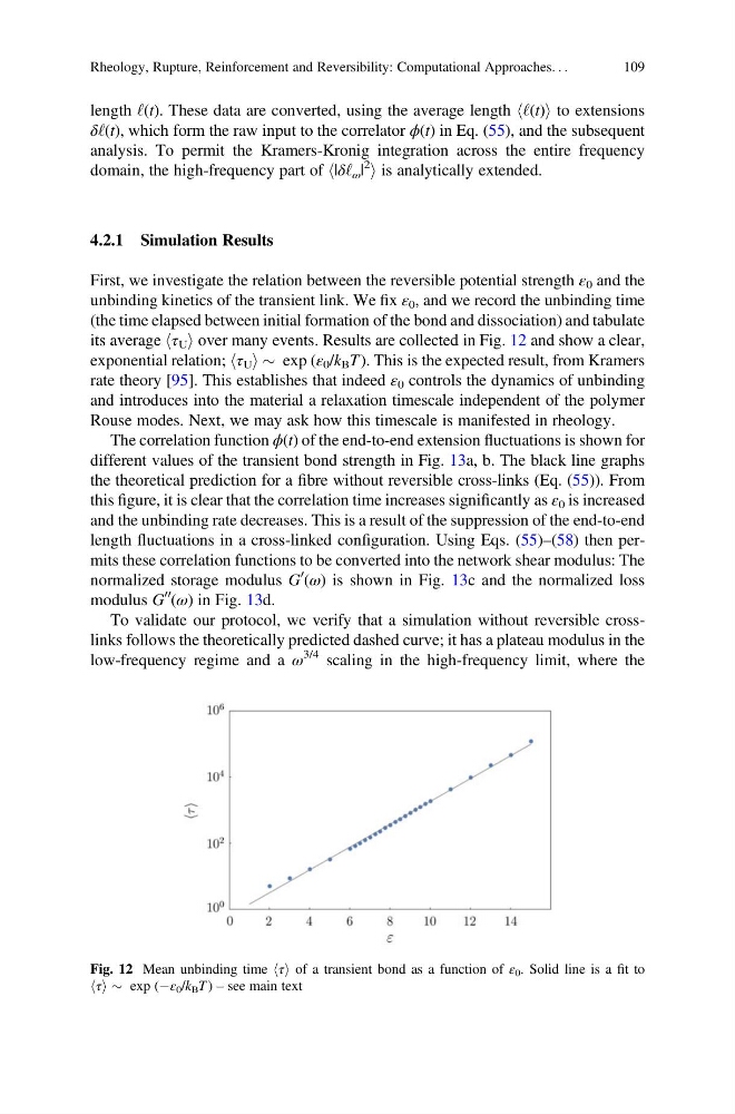
unbinding kinetics of the transient link. We fix ε 0 , and we record the unbinding time
(the time elapsed between initial formation of the bond and dissociation) and tabulate
its average hτ U i over many events. Results are collected in Fig. 12 and show a clear,
exponential relation; hτ U i $ exp (ε 0 /k B T). This is the expected result, from Kramers
rate theory [95]. This establishes that indeed ε 0 controls the dynamics of unbinding
and introduces into the material a relaxation timescale independent of the polymer
Rouse modes. Next, we may ask how this timescale is manifested in rheology.
The correlation function ϕ(t) of the end-to-end extension fluctuations is shown for
different values of the transient bond strength in Fig. 13a, b. The black line graphs
the theoretical prediction for a fibre without reversible cross-links (Eq. (55)). From
this figure, it is clear that the correlation time increases significantly as ε 0 is increased
and the unbinding rate decreases. This is a result of the suppression of the end-to-end
length fluctuations in a cross-linked configuration. Using Eqs. (55)–(58) then permits these correlation functions to be converted into the network shear modulus: The
normalized storage modulus G
0 (ω) is shown in Fig. 13c and the normalized loss
modulus G
00 (ω) in Fig. 13d.
To validate our protocol, we verify that a simulation without reversible crosslinks follows the theoretically predicted dashed curve; it has a plateau modulus in the
low-frequency regime and a ω
3/4 scaling in the high-frequency limit, where the
Fig. 12 Mean unbinding time hτi of a transient bond as a function of ε 0 . Solid line is a fit to
hτi $ exp (Àε 0 /k B T ) – see main text
Rheology, Rupture, Reinforcement and Reversibility: Computational Approaches. . .
109
δ‘(t), which form the raw input to the correlator ϕ(t) in Eq. (55), and the subsequent
analysis. To permit the Kramers-Kronig integration across the entire frequency
domain, the high-frequency part of h|δ‘ ω |
2
i is analytically extended.
4.2.1 Simulation Results
First, we investigate the relation between the reversible potential strength ε 0 and the
unbinding kinetics of the transient link. We fix ε 0 , and we record the unbinding time
(the time elapsed between initial formation of the bond and dissociation) and tabulate
its average hτ U i over many events. Results are collected in Fig. 12 and show a clear,
exponential relation; hτ U i $ exp (ε 0 /k B T). This is the expected result, from Kramers
rate theory [95]. This establishes that indeed ε 0 controls the dynamics of unbinding
and introduces into the material a relaxation timescale independent of the polymer
Rouse modes. Next, we may ask how this timescale is manifested in rheology.
The correlation function ϕ(t) of the end-to-end extension fluctuations is shown for
different values of the transient bond strength in Fig. 13a, b. The black line graphs
the theoretical prediction for a fibre without reversible cross-links (Eq. (55)). From
this figure, it is clear that the correlation time increases significantly as ε 0 is increased
and the unbinding rate decreases. This is a result of the suppression of the end-to-end
length fluctuations in a cross-linked configuration. Using Eqs. (55)–(58) then permits these correlation functions to be converted into the network shear modulus: The
normalized storage modulus G
0 (ω) is shown in Fig. 13c and the normalized loss
modulus G
00 (ω) in Fig. 13d.
To validate our protocol, we verify that a simulation without reversible crosslinks follows the theoretically predicted dashed curve; it has a plateau modulus in the
low-frequency regime and a ω
3/4 scaling in the high-frequency limit, where the
Fig. 12 Mean unbinding time hτi of a transient bond as a function of ε 0 . Solid line is a fit to
hτi $ exp (Àε 0 /k B T ) – see main text
Rheology, Rupture, Reinforcement and Reversibility: Computational Approaches. . .
109