

reversible cross-link simulation. This suggests that neither the strong- nor weakbinding reversible cross-links influence the spatial structure between the permanent
cross-links themselves.
4.2 Dynamic Bulk Rheology of Reversibly Linked Materials
In this section, we apply the simulational concepts laid out in Sect. 3.5.1 to predict
the frequency-dependent rheology of a polymer material (elastomeric or hydrogel)
containing both permanent and reversible links.
In the simulations presented here, we focus on the effects of changing the binding
strength depth on the dynamic rheology. To compare apples and apples, we fix a
number of other parameters. Throughout the simulations, we fixed k B T ¼ 1 and
m ¼ 1. Parameters defining the geometry of the polymers were N ¼ 42, and d ¼ 1
(in MD length units). Only one in six beads is capable of forming a reversible bond.
The elastic energy of the chain was fixed by choosing x 0 ¼ 1 and K sp ¼ 2, 500 (this
extremely high value suppresses bond length fluctuations, rendering the chain
effectively inextensible) and K b ¼ 15, corresponding to a persistence length
‘ p ¼ 30. The single-bead friction coefficient was fixed at γ ¼ 0.1.
The rebinding kinetics are independent of the transient potential, as these are
determined by the encounter rate between transient binding partners in the network.
As such, these depend most strongly on the density ρ. By fixing hτ R i ¼ 200, we
ensure that we work, approximately, at fixed network density.
In our simulations, one end of the polymer is fixed at the origin – this represents
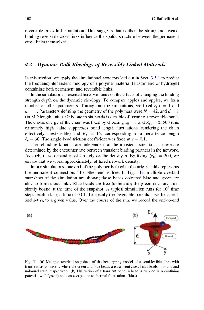
the permanent connection. The other end is free. In Fig. 11a, multiple overlaid
snapshots of the simulation are shown; those beads coloured blue and green are
able to form cross-links. Blue beads are free (unbound); the green ones are transiently bound at the time of the snapshot. A typical simulation runs for 10
9 time
steps, each taking a time of 0.01. To specify the reversible potential, we fix r c ¼ 1
and set ε 0 to a given value. Over the course of the run, we record the end-to-end
Fig. 11 (a) Multiple overlaid snapshots of the bead-spring model of a semiflexible fibre with
transient cross-linkers, where the green and blue beads are transient cross-links beads in bound and
unbound state, respectively. (b) Illustration of a transient bond, a bead is trapped in a confining
potential well (green) and can escape due to thermal fluctuations (blue)
108
C. Raffaelli et al.
cross-links themselves.
4.2 Dynamic Bulk Rheology of Reversibly Linked Materials
In this section, we apply the simulational concepts laid out in Sect. 3.5.1 to predict
the frequency-dependent rheology of a polymer material (elastomeric or hydrogel)
containing both permanent and reversible links.
In the simulations presented here, we focus on the effects of changing the binding
strength depth on the dynamic rheology. To compare apples and apples, we fix a
number of other parameters. Throughout the simulations, we fixed k B T ¼ 1 and
m ¼ 1. Parameters defining the geometry of the polymers were N ¼ 42, and d ¼ 1
(in MD length units). Only one in six beads is capable of forming a reversible bond.
The elastic energy of the chain was fixed by choosing x 0 ¼ 1 and K sp ¼ 2, 500 (this
extremely high value suppresses bond length fluctuations, rendering the chain
effectively inextensible) and K b ¼ 15, corresponding to a persistence length
‘ p ¼ 30. The single-bead friction coefficient was fixed at γ ¼ 0.1.
The rebinding kinetics are independent of the transient potential, as these are
determined by the encounter rate between transient binding partners in the network.
As such, these depend most strongly on the density ρ. By fixing hτ R i ¼ 200, we
ensure that we work, approximately, at fixed network density.
In our simulations, one end of the polymer is fixed at the origin – this represents
the permanent connection. The other end is free. In Fig. 11a, multiple overlaid
snapshots of the simulation are shown; those beads coloured blue and green are
able to form cross-links. Blue beads are free (unbound); the green ones are transiently bound at the time of the snapshot. A typical simulation runs for 10
9 time
steps, each taking a time of 0.01. To specify the reversible potential, we fix r c ¼ 1
and set ε 0 to a given value. Over the course of the run, we record the end-to-end
Fig. 11 (a) Multiple overlaid snapshots of the bead-spring model of a semiflexible fibre with
transient cross-linkers, where the green and blue beads are transient cross-links beads in bound and
unbound state, respectively. (b) Illustration of a transient bond, a bead is trapped in a confining
potential well (green) and can escape due to thermal fluctuations (blue)
108
C. Raffaelli et al.