

ϕ t
ð Þ ¼ δℓ t
ð Þδℓ 0
ð Þ
h
i
ð55Þ
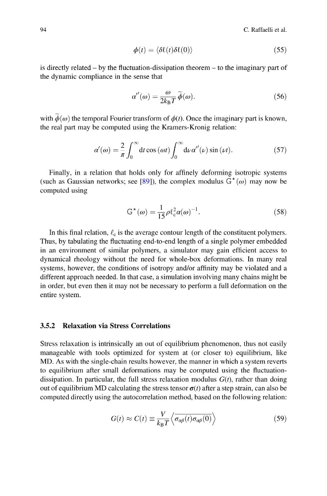
is directly related – by the fluctuation-dissipation theorem – to the imaginary part of
the dynamic compliance in the sense that
α
0 0 ω
ð Þ ¼
ω
2k B T
e
ϕ ω
ð Þ:
ð56Þ
with e
ϕ ω
ð Þ the temporal Fourier transform of ϕ(t). Once the imaginary part is known,
the real part may be computed using the Kramers-Kronig relation:
α
0
ω
ð Þ ¼
2
π
Z 1
0
dt cos ωt
ð Þ
Z 1
0
dνα
0 0 ν
ð Þ sin νt
ð Þ:
ð57Þ
Finally, in a relation that holds only for affinely deforming isotropic systems
(such as Gaussian networks; see [89]), the complex modulus G
⋆ ω
ð Þ may now be
computed using
G
⋆ ω
ð Þ ¼
1
15
ρℓ
2
c α ω
ð Þ
À1 :
ð58Þ
In this final relation, ‘ c is the average contour length of the constituent polymers.
Thus, by tabulating the fluctuating end-to-end length of a single polymer embedded
in an environment of similar polymers, a simulator may gain efficient access to
dynamical rheology without the need for whole-box deformations. In many real
systems, however, the conditions of isotropy and/or affinity may be violated and a
different approach needed. In that case, a simulation involving many chains might be
in order, but even then it may not be necessary to perform a full deformation on the
entire system.
3.5.2 Relaxation via Stress Correlations
Stress relaxation is intrinsically an out of equilibrium phenomenon, thus not easily
manageable with tools optimized for system at (or closer to) equilibrium, like
MD. As with the single-chain results however, the manner in which a system reverts
to equilibrium after small deformations may be computed using the fluctuationdissipation. In particular, the full stress relaxation modulus G(t), rather than doing
out of equilibrium MD calculating the stress tensor σ(t) after a step strain, can also be
computed directly using the autocorrelation method, based on the following relation:
G t
ð Þ % C t
ð Þ
V
k B T
σ αβ t
ð Þσ αβ 0
ð Þ
D
E
ð59Þ
94
C. Raffaelli et al.
ð Þ ¼ δℓ t
ð Þδℓ 0
ð Þ
h
i
ð55Þ
is directly related – by the fluctuation-dissipation theorem – to the imaginary part of
the dynamic compliance in the sense that
α
0 0 ω
ð Þ ¼
ω
2k B T
e
ϕ ω
ð Þ:
ð56Þ
with e
ϕ ω
ð Þ the temporal Fourier transform of ϕ(t). Once the imaginary part is known,
the real part may be computed using the Kramers-Kronig relation:
α
0
ω
ð Þ ¼
2
π
Z 1
0
dt cos ωt
ð Þ
Z 1
0
dνα
0 0 ν
ð Þ sin νt
ð Þ:
ð57Þ
Finally, in a relation that holds only for affinely deforming isotropic systems
(such as Gaussian networks; see [89]), the complex modulus G
⋆ ω
ð Þ may now be
computed using
G
⋆ ω
ð Þ ¼
1
15
ρℓ
2
c α ω
ð Þ
À1 :
ð58Þ
In this final relation, ‘ c is the average contour length of the constituent polymers.
Thus, by tabulating the fluctuating end-to-end length of a single polymer embedded
in an environment of similar polymers, a simulator may gain efficient access to
dynamical rheology without the need for whole-box deformations. In many real
systems, however, the conditions of isotropy and/or affinity may be violated and a
different approach needed. In that case, a simulation involving many chains might be
in order, but even then it may not be necessary to perform a full deformation on the
entire system.
3.5.2 Relaxation via Stress Correlations
Stress relaxation is intrinsically an out of equilibrium phenomenon, thus not easily
manageable with tools optimized for system at (or closer to) equilibrium, like
MD. As with the single-chain results however, the manner in which a system reverts
to equilibrium after small deformations may be computed using the fluctuationdissipation. In particular, the full stress relaxation modulus G(t), rather than doing
out of equilibrium MD calculating the stress tensor σ(t) after a step strain, can also be
computed directly using the autocorrelation method, based on the following relation:
G t
ð Þ % C t
ð Þ
V
k B T
σ αβ t
ð Þσ αβ 0
ð Þ
D
E
ð59Þ
94
C. Raffaelli et al.