

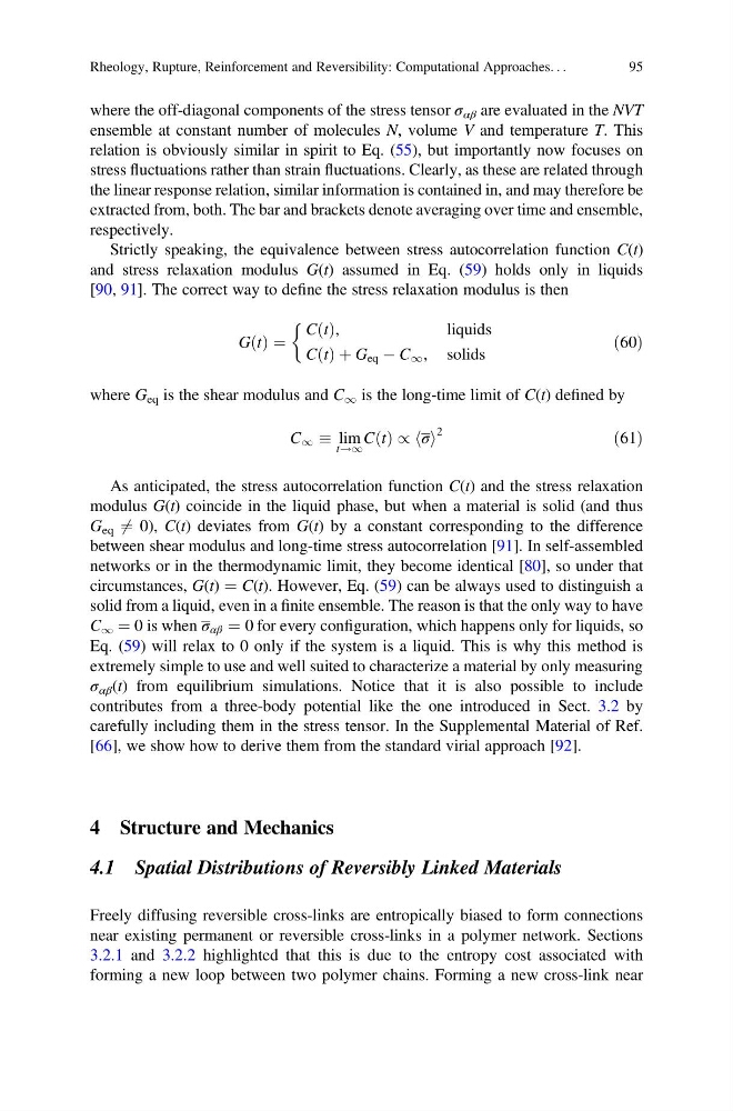
where the off-diagonal components of the stress tensor σ αβ are evaluated in the NVT
ensemble at constant number of molecules N, volume V and temperature T. This
relation is obviously similar in spirit to Eq. (55), but importantly now focuses on
stress fluctuations rather than strain fluctuations. Clearly, as these are related through
the linear response relation, similar information is contained in, and may therefore be
extracted from, both. The bar and brackets denote averaging over time and ensemble,
respectively.
Strictly speaking, the equivalence between stress autocorrelation function C(t)
and stress relaxation modulus G(t) assumed in Eq. (59) holds only in liquids
[90, 91]. The correct way to define the stress relaxation modulus is then
G t
ð Þ ¼
C t
ð Þ,
liquids
C t
ð Þ þ G eq À C 1 , solids
&
ð60Þ
where G eq is the shear modulus and C 1 is the long-time limit of C(t) defined by
C 1 lim
t!1
C t
ð Þ / σ
h i
2
ð61Þ
As anticipated, the stress autocorrelation function C(t) and the stress relaxation
modulus G(t) coincide in the liquid phase, but when a material is solid (and thus
G eq 6 ¼ 0), C(t) deviates from G(t) by a constant corresponding to the difference
between shear modulus and long-time stress autocorrelation [91]. In self-assembled
networks or in the thermodynamic limit, they become identical [80], so under that
circumstances, G(t) ¼ C(t). However, Eq. (59) can be always used to distinguish a
solid from a liquid, even in a finite ensemble. The reason is that the only way to have
C 1 ¼ 0 is when σ αβ ¼ 0 for every configuration, which happens only for liquids, so
Eq. (59) will relax to 0 only if the system is a liquid. This is why this method is
extremely simple to use and well suited to characterize a material by only measuring
σ αβ (t) from equilibrium simulations. Notice that it is also possible to include
contributes from a three-body potential like the one introduced in Sect. 3.2 by
carefully including them in the stress tensor. In the Supplemental Material of Ref.
[66], we show how to derive them from the standard virial approach [92].
4 Structure and Mechanics
4.1 Spatial Distributions of Reversibly Linked Materials
Freely diffusing reversible cross-links are entropically biased to form connections
near existing permanent or reversible cross-links in a polymer network. Sections
3.2.1 and 3.2.2 highlighted that this is due to the entropy cost associated with
forming a new loop between two polymer chains. Forming a new cross-link near
Rheology, Rupture, Reinforcement and Reversibility: Computational Approaches. . .
95
ensemble at constant number of molecules N, volume V and temperature T. This
relation is obviously similar in spirit to Eq. (55), but importantly now focuses on
stress fluctuations rather than strain fluctuations. Clearly, as these are related through
the linear response relation, similar information is contained in, and may therefore be
extracted from, both. The bar and brackets denote averaging over time and ensemble,
respectively.
Strictly speaking, the equivalence between stress autocorrelation function C(t)
and stress relaxation modulus G(t) assumed in Eq. (59) holds only in liquids
[90, 91]. The correct way to define the stress relaxation modulus is then
G t
ð Þ ¼
C t
ð Þ,
liquids
C t
ð Þ þ G eq À C 1 , solids
&
ð60Þ
where G eq is the shear modulus and C 1 is the long-time limit of C(t) defined by
C 1 lim
t!1
C t
ð Þ / σ
h i
2
ð61Þ
As anticipated, the stress autocorrelation function C(t) and the stress relaxation
modulus G(t) coincide in the liquid phase, but when a material is solid (and thus
G eq 6 ¼ 0), C(t) deviates from G(t) by a constant corresponding to the difference
between shear modulus and long-time stress autocorrelation [91]. In self-assembled
networks or in the thermodynamic limit, they become identical [80], so under that
circumstances, G(t) ¼ C(t). However, Eq. (59) can be always used to distinguish a
solid from a liquid, even in a finite ensemble. The reason is that the only way to have
C 1 ¼ 0 is when σ αβ ¼ 0 for every configuration, which happens only for liquids, so
Eq. (59) will relax to 0 only if the system is a liquid. This is why this method is
extremely simple to use and well suited to characterize a material by only measuring
σ αβ (t) from equilibrium simulations. Notice that it is also possible to include
contributes from a three-body potential like the one introduced in Sect. 3.2 by
carefully including them in the stress tensor. In the Supplemental Material of Ref.
[66], we show how to derive them from the standard virial approach [92].
4 Structure and Mechanics
4.1 Spatial Distributions of Reversibly Linked Materials
Freely diffusing reversible cross-links are entropically biased to form connections
near existing permanent or reversible cross-links in a polymer network. Sections
3.2.1 and 3.2.2 highlighted that this is due to the entropy cost associated with
forming a new loop between two polymer chains. Forming a new cross-link near
Rheology, Rupture, Reinforcement and Reversibility: Computational Approaches. . .
95