

Random Spacing Model
147
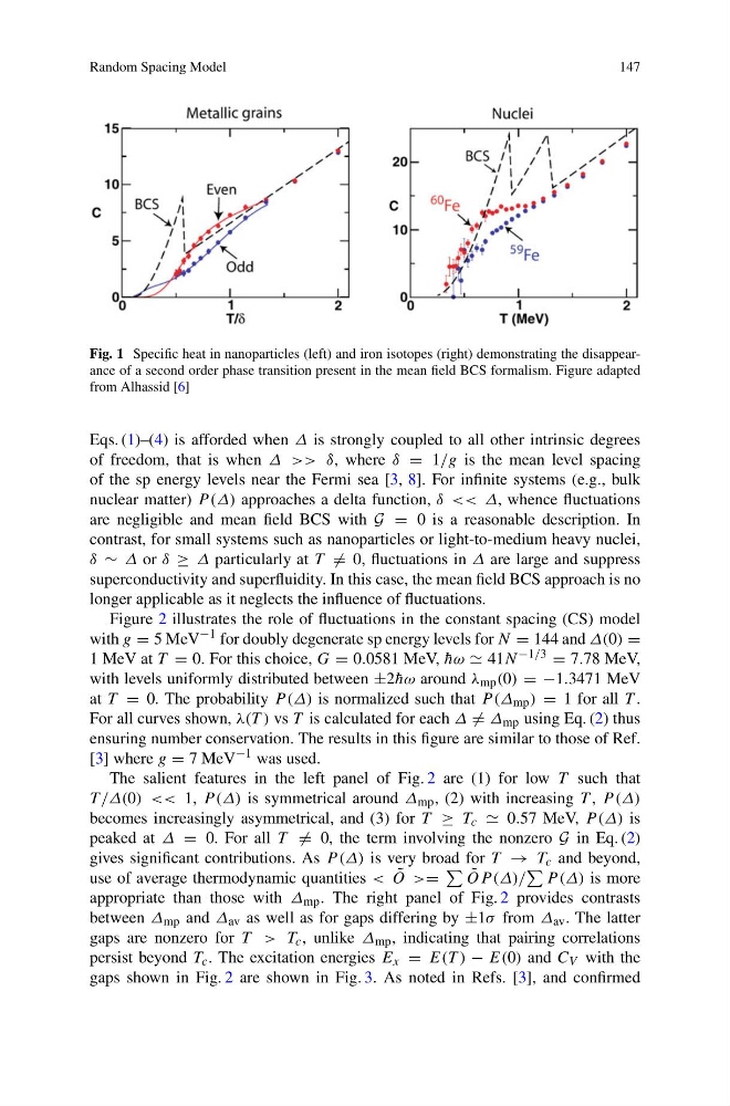
Fig. 1 Specific heat in nanoparticles (left) and iron isotopes (right) demonstrating the disappearance of a second order phase transition present in the mean field BCS formalism. Figure adapted
from Alhassid [6]
Eqs. (1)–(4) is afforded when Δ is strongly coupled to all other intrinsic degrees
of freedom, that is when Δ >> δ, where δ = 1/g is the mean level spacing
of the sp energy levels near the Fermi sea [3, 8]. For infinite systems (e.g., bulk
nuclear matter) P (Δ) approaches a delta function, δ << Δ, whence fluctuations
are negligible and mean field BCS with G = 0 is a reasonable description. In
contrast, for small systems such as nanoparticles or light-to-medium heavy nuclei,
δ ∼ Δ or δ ≥ Δ particularly at T = 0, fluctuations in Δ are large and suppress
superconductivity and superfluidity. In this case, the mean field BCS approach is no
longer applicable as it neglects the influence of fluctuations.
Figure 2 illustrates the role of fluctuations in the constant spacing (CS) model
with g = 5 MeV
−1 for doubly degenerate sp energy levels for N = 144 and Δ(0) =
1 MeV at T = 0. For this choice, G = 0.0581 MeV, ¯
hω 41N −1/3 = 7.78 MeV,
with levels uniformly distributed between ±2 ¯
hω around λ mp (0) = −1.3471 MeV
at T = 0. The probability P (Δ) is normalized such that P (Δ mp ) = 1 for all T .
For all curves shown, λ(T ) vs T is calculated for each Δ = Δ mp using Eq. (2) thus
ensuring number conservation. The results in this figure are similar to those of Ref.
[3] where g = 7 MeV
−1 was used.
The salient features in the left panel of Fig. 2 are (1) for low T such that
T /Δ(0) << 1, P (Δ) is symmetrical around Δ mp , (2) with increasing T , P (Δ)
becomes increasingly asymmetrical, and (3) for T ≥ T c 0.57 MeV, P (Δ) is
peaked at Δ = 0. For all T = 0, the term involving the nonzero G in Eq. (2)
gives significant contributions. As P (Δ) is very broad for T → T c and beyond,
use of average thermodynamic quantities < ˜
O >=
˜
OP (Δ)/
P (Δ) is more
appropriate than those with Δ mp . The right panel of Fig. 2 provides contrasts
between Δ mp and Δ av as well as for gaps differing by ±1σ from Δ av . The latter
gaps are nonzero for T > T c , unlike Δ mp , indicating that pairing correlations
persist beyond T c . The excitation energies E x = E(T ) − E(0) and C V with the
gaps shown in Fig. 2 are shown in Fig. 3. As noted in Refs. [3], and confirmed
147
Fig. 1 Specific heat in nanoparticles (left) and iron isotopes (right) demonstrating the disappearance of a second order phase transition present in the mean field BCS formalism. Figure adapted
from Alhassid [6]
Eqs. (1)–(4) is afforded when Δ is strongly coupled to all other intrinsic degrees
of freedom, that is when Δ >> δ, where δ = 1/g is the mean level spacing
of the sp energy levels near the Fermi sea [3, 8]. For infinite systems (e.g., bulk
nuclear matter) P (Δ) approaches a delta function, δ << Δ, whence fluctuations
are negligible and mean field BCS with G = 0 is a reasonable description. In
contrast, for small systems such as nanoparticles or light-to-medium heavy nuclei,
δ ∼ Δ or δ ≥ Δ particularly at T = 0, fluctuations in Δ are large and suppress
superconductivity and superfluidity. In this case, the mean field BCS approach is no
longer applicable as it neglects the influence of fluctuations.
Figure 2 illustrates the role of fluctuations in the constant spacing (CS) model
with g = 5 MeV
−1 for doubly degenerate sp energy levels for N = 144 and Δ(0) =
1 MeV at T = 0. For this choice, G = 0.0581 MeV, ¯
hω 41N −1/3 = 7.78 MeV,
with levels uniformly distributed between ±2 ¯
hω around λ mp (0) = −1.3471 MeV
at T = 0. The probability P (Δ) is normalized such that P (Δ mp ) = 1 for all T .
For all curves shown, λ(T ) vs T is calculated for each Δ = Δ mp using Eq. (2) thus
ensuring number conservation. The results in this figure are similar to those of Ref.
[3] where g = 7 MeV
−1 was used.
The salient features in the left panel of Fig. 2 are (1) for low T such that
T /Δ(0) << 1, P (Δ) is symmetrical around Δ mp , (2) with increasing T , P (Δ)
becomes increasingly asymmetrical, and (3) for T ≥ T c 0.57 MeV, P (Δ) is
peaked at Δ = 0. For all T = 0, the term involving the nonzero G in Eq. (2)
gives significant contributions. As P (Δ) is very broad for T → T c and beyond,
use of average thermodynamic quantities < ˜
O >=
˜
OP (Δ)/
P (Δ) is more
appropriate than those with Δ mp . The right panel of Fig. 2 provides contrasts
between Δ mp and Δ av as well as for gaps differing by ±1σ from Δ av . The latter
gaps are nonzero for T > T c , unlike Δ mp , indicating that pairing correlations
persist beyond T c . The excitation energies E x = E(T ) − E(0) and C V with the
gaps shown in Fig. 2 are shown in Fig. 3. As noted in Refs. [3], and confirmed