

128
V. Zelevinsky and S. Karampagia
10 11 12 13 14 15 16 17 18 19
Neutron Number
3.2
3.4
3.6
3.8
4
4.2
4.4
4.6
4.8
5
Temperature (MeV)
10 11 12 13 14 15 16 17 18 19
Neutron Number
3.2
3.4
3.6
3.8
4
4.2
4.4
4.6
4.8
5
Temperature (MeV)
10 11 12 13 14 15 16 17 18 19
Neutron Number
3.2
3.4
3.6
3.8
4
4.2
4.4
4.6
4.8
5
Temperature (MeV)
m
u
n
i
m
u
l
A
m
u
i
s
e
n
g
a
M
Silicon
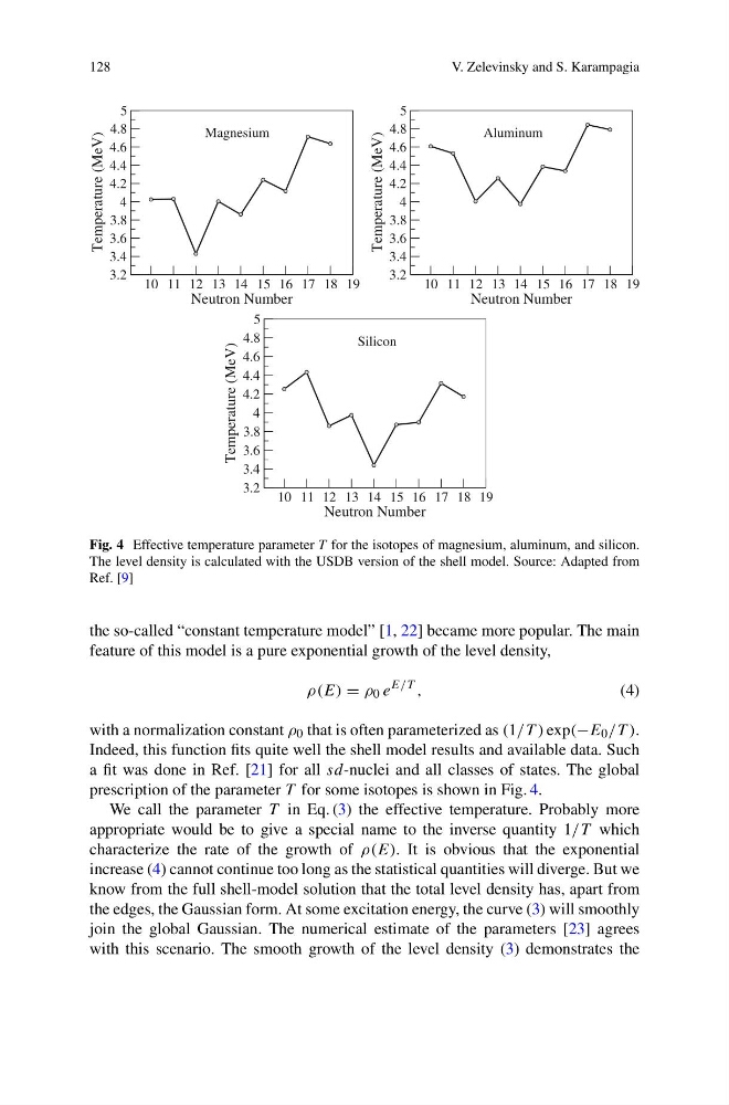
Fig. 4 Effective temperature parameter T for the isotopes of magnesium, aluminum, and silicon.
The level density is calculated with the USDB version of the shell model. Source: Adapted from
Ref. [9]
the so-called “constant temperature model” [1, 22] became more popular. The main
feature of this model is a pure exponential growth of the level density,
ρ(E) = ρ 0 e
E/T ,
(4)
with a normalization constant ρ 0 that is often parameterized as (1/T ) exp(−E 0 /T ).
Indeed, this function fits quite well the shell model results and available data. Such
a fit was done in Ref. [21] for all sd-nuclei and all classes of states. The global
prescription of the parameter T for some isotopes is shown in Fig. 4.
We call the parameter T in Eq. (3) the effective temperature. Probably more
appropriate would be to give a special name to the inverse quantity 1/T which
characterize the rate of the growth of ρ(E). It is obvious that the exponential
increase (4) cannot continue too long as the statistical quantities will diverge. But we
know from the full shell-model solution that the total level density has, apart from
the edges, the Gaussian form. At some excitation energy, the curve (3) will smoothly
join the global Gaussian. The numerical estimate of the parameters [23] agrees
with this scenario. The smooth growth of the level density (3) demonstrates the
V. Zelevinsky and S. Karampagia
10 11 12 13 14 15 16 17 18 19
Neutron Number
3.2
3.4
3.6
3.8
4
4.2
4.4
4.6
4.8
5
Temperature (MeV)
10 11 12 13 14 15 16 17 18 19
Neutron Number
3.2
3.4
3.6
3.8
4
4.2
4.4
4.6
4.8
5
Temperature (MeV)
10 11 12 13 14 15 16 17 18 19
Neutron Number
3.2
3.4
3.6
3.8
4
4.2
4.4
4.6
4.8
5
Temperature (MeV)
m
u
n
i
m
u
l
A
m
u
i
s
e
n
g
a
M
Silicon
Fig. 4 Effective temperature parameter T for the isotopes of magnesium, aluminum, and silicon.
The level density is calculated with the USDB version of the shell model. Source: Adapted from
Ref. [9]
the so-called “constant temperature model” [1, 22] became more popular. The main
feature of this model is a pure exponential growth of the level density,
ρ(E) = ρ 0 e
E/T ,
(4)
with a normalization constant ρ 0 that is often parameterized as (1/T ) exp(−E 0 /T ).
Indeed, this function fits quite well the shell model results and available data. Such
a fit was done in Ref. [21] for all sd-nuclei and all classes of states. The global
prescription of the parameter T for some isotopes is shown in Fig. 4.
We call the parameter T in Eq. (3) the effective temperature. Probably more
appropriate would be to give a special name to the inverse quantity 1/T which
characterize the rate of the growth of ρ(E). It is obvious that the exponential
increase (4) cannot continue too long as the statistical quantities will diverge. But we
know from the full shell-model solution that the total level density has, apart from
the edges, the Gaussian form. At some excitation energy, the curve (3) will smoothly
join the global Gaussian. The numerical estimate of the parameters [23] agrees
with this scenario. The smooth growth of the level density (3) demonstrates the