

Nuclear Shell Model and Level Density
127
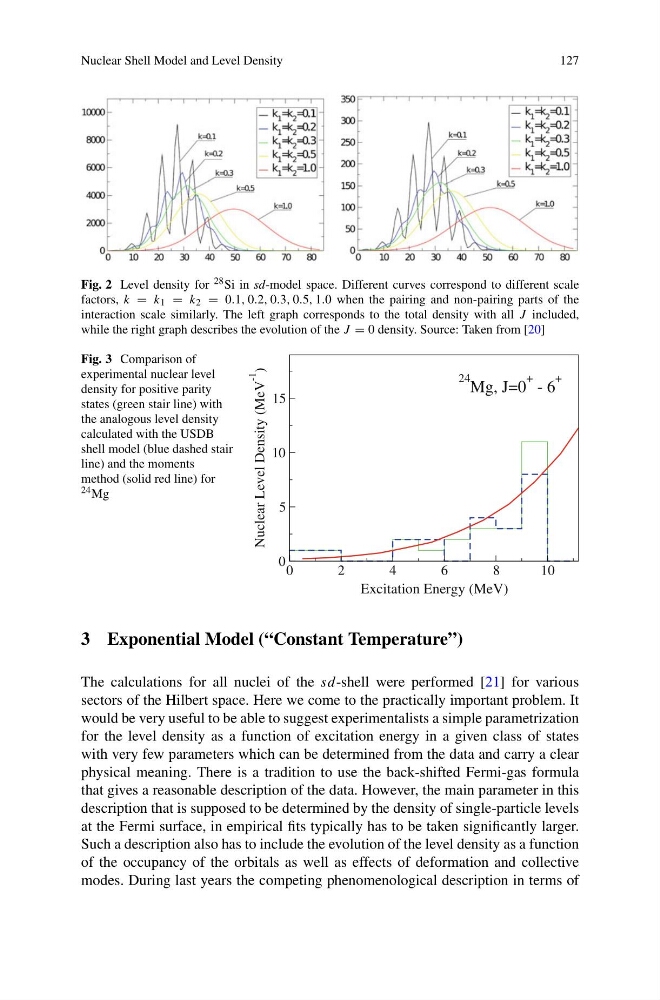
Fig. 2 Level density for 28 Si in sd-model space. Different curves correspond to different scale
factors, k = k 1 = k 2 = 0.1, 0.2, 0.3, 0.5, 1.0 when the pairing and non-pairing parts of the
interaction scale similarly. The left graph corresponds to the total density with all J included,
while the right graph describes the evolution of the J = 0 density. Source: Taken from [20]
Fig. 3 Comparison of
experimental nuclear level
density for positive parity
states (green stair line) with
the analogous level density
calculated with the USDB
shell model (blue dashed stair
line) and the moments
method (solid red line) for
24 Mg
0
2
4
6
8
1 0
Excitation Energy (MeV)
0
5
10
15
Nuclear Level Density (MeV
-1
)
24
Mg, J=0
+ - 6
+
3 Exponential Model (“Constant Temperature”)
The calculations for all nuclei of the sd-shell were performed [21] for various
sectors of the Hilbert space. Here we come to the practically important problem. It
would be very useful to be able to suggest experimentalists a simple parametrization
for the level density as a function of excitation energy in a given class of states
with very few parameters which can be determined from the data and carry a clear
physical meaning. There is a tradition to use the back-shifted Fermi-gas formula
that gives a reasonable description of the data. However, the main parameter in this
description that is supposed to be determined by the density of single-particle levels
at the Fermi surface, in empirical fits typically has to be taken significantly larger.
Such a description also has to include the evolution of the level density as a function
of the occupancy of the orbitals as well as effects of deformation and collective
modes. During last years the competing phenomenological description in terms of
127
Fig. 2 Level density for 28 Si in sd-model space. Different curves correspond to different scale
factors, k = k 1 = k 2 = 0.1, 0.2, 0.3, 0.5, 1.0 when the pairing and non-pairing parts of the
interaction scale similarly. The left graph corresponds to the total density with all J included,
while the right graph describes the evolution of the J = 0 density. Source: Taken from [20]
Fig. 3 Comparison of
experimental nuclear level
density for positive parity
states (green stair line) with
the analogous level density
calculated with the USDB
shell model (blue dashed stair
line) and the moments
method (solid red line) for
24 Mg
0
2
4
6
8
1 0
Excitation Energy (MeV)
0
5
10
15
Nuclear Level Density (MeV
-1
)
24
Mg, J=0
+ - 6
+
3 Exponential Model (“Constant Temperature”)
The calculations for all nuclei of the sd-shell were performed [21] for various
sectors of the Hilbert space. Here we come to the practically important problem. It
would be very useful to be able to suggest experimentalists a simple parametrization
for the level density as a function of excitation energy in a given class of states
with very few parameters which can be determined from the data and carry a clear
physical meaning. There is a tradition to use the back-shifted Fermi-gas formula
that gives a reasonable description of the data. However, the main parameter in this
description that is supposed to be determined by the density of single-particle levels
at the Fermi surface, in empirical fits typically has to be taken significantly larger.
Such a description also has to include the evolution of the level density as a function
of the occupancy of the orbitals as well as effects of deformation and collective
modes. During last years the competing phenomenological description in terms of