

17 A Framework for Dynamic Simulation of Interconnected …
609
• if the number or composition of the distributed parameters varies, the model itself
must track these changes and correctly respond to them;
• the model should ensure the setting of all distributions defined at the input into
the output flows, even those that are not explicitly considered in its equations.
It can be concluded that the commonly used explicit approach is not applicable for
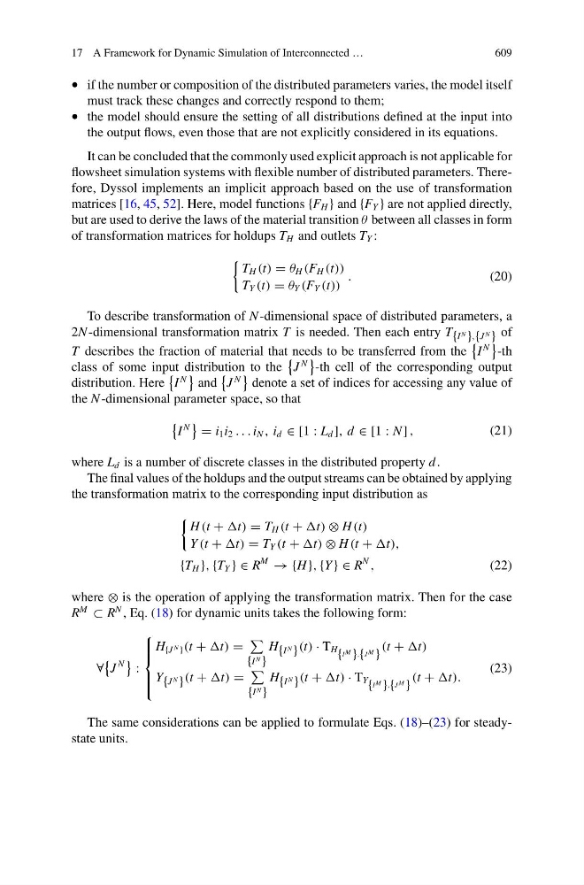
flowsheet simulation systems with flexible number of distributed parameters. Therefore, Dyssol implements an implicit approach based on the use of transformation
matrices [16, 45, 52]. Here, model functions {F H } and {F Y } are not applied directly,
but are used to derive the laws of the material transition θ between all classes in form
of transformation matrices for holdups T H and outlets T Y :
T H (t) = θ H (F H (t))
T Y (t) = θ Y (F Y (t))
.
(20)
To describe transformation of N -dimensional space of distributed parameters, a
2N -dimensional transformation matrix T is needed. Then each entry T {I
N
},{J
N
} of
T describes the fraction of material that needs to be transferred from the
I
N
-th
class of some input distribution to the
J
N
-th cell of the corresponding output
distribution. Here
I
N
and
J
N
denote a set of indices for accessing any value of
the N -dimensional parameter space, so that
I
N
= i 1 i 2 . . . i N , i d ∈ [1 : L d ], d ∈ [1 : N ] ,
(21)
where L d is a number of discrete classes in the distributed property d .
The final values of the holdups and the output streams can be obtained by applying
the transformation matrix to the corresponding input distribution as
H (t + t) = T H (t + t) ⊗ H (t)
Y (t + t) = T Y (t + t) ⊗ H (t + t),
{T H }, {T Y } ∈ R
M
→ {H }, {Y } ∈ R
N
,
(22)
where ⊗ is the operation of applying the transformation matrix. Then for the case
R
M
⊂ R
N , Eq. (18) for dynamic units takes the following form:
∀
J
N
:
⎧
⎪ ⎪ ⎨
⎪ ⎪ ⎩
H {J N } (t + t) =
{I
N
}
H {I
N
} (t) · T H { I M } , { J M }
(t + t)
Y {J
N
} (t + t) =
{I
N
}
H {I
N
} (t + t) · T Y { I M } , { J M }
(t + t).
(23)
The same considerations can be applied to formulate Eqs. (18)–(23) for steadystate units.
609
• if the number or composition of the distributed parameters varies, the model itself
must track these changes and correctly respond to them;
• the model should ensure the setting of all distributions defined at the input into
the output flows, even those that are not explicitly considered in its equations.
It can be concluded that the commonly used explicit approach is not applicable for
flowsheet simulation systems with flexible number of distributed parameters. Therefore, Dyssol implements an implicit approach based on the use of transformation
matrices [16, 45, 52]. Here, model functions {F H } and {F Y } are not applied directly,
but are used to derive the laws of the material transition θ between all classes in form
of transformation matrices for holdups T H and outlets T Y :
T H (t) = θ H (F H (t))
T Y (t) = θ Y (F Y (t))
.
(20)
To describe transformation of N -dimensional space of distributed parameters, a
2N -dimensional transformation matrix T is needed. Then each entry T {I
N
},{J
N
} of
T describes the fraction of material that needs to be transferred from the
I
N
-th
class of some input distribution to the
J
N
-th cell of the corresponding output
distribution. Here
I
N
and
J
N
denote a set of indices for accessing any value of
the N -dimensional parameter space, so that
I
N
= i 1 i 2 . . . i N , i d ∈ [1 : L d ], d ∈ [1 : N ] ,
(21)
where L d is a number of discrete classes in the distributed property d .
The final values of the holdups and the output streams can be obtained by applying
the transformation matrix to the corresponding input distribution as
H (t + t) = T H (t + t) ⊗ H (t)
Y (t + t) = T Y (t + t) ⊗ H (t + t),
{T H }, {T Y } ∈ R
M
→ {H }, {Y } ∈ R
N
,
(22)
where ⊗ is the operation of applying the transformation matrix. Then for the case
R
M
⊂ R
N , Eq. (18) for dynamic units takes the following form:
∀
J
N
:
⎧
⎪ ⎪ ⎨
⎪ ⎪ ⎩
H {J N } (t + t) =
{I
N
}
H {I
N
} (t) · T H { I M } , { J M }
(t + t)
Y {J
N
} (t + t) =
{I
N
}
H {I
N
} (t + t) · T Y { I M } , { J M }
(t + t).
(23)
The same considerations can be applied to formulate Eqs. (18)–(23) for steadystate units.