

608
V. Skorych et al.
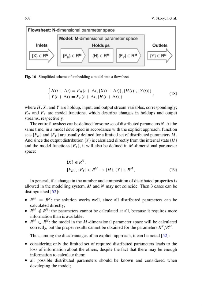
Fig. 16 Simplified scheme of embedding a model into a flowsheet
H (t + t) = F H (t + t, {X (t + t)}, {H (t)}, {Y (t)})
Y (t + t) = F Y (t + t, {H (t + t)})
,
(18)
where H , X , and Y are holdup, input, and output stream variables, correspondingly;
F H and F Y are model functions, which describe changes in holdups and output
streams, respectively.
The entire flowsheet can be defined for some set of distributed parameters N . At the
same time, in a model developed in accordance with the explicit approach, function
sets {F H } and {F Y } are usually defined for a limited set of distributed parameters M .
And since the output distribution {Y } is calculated directly from the internal state {H }
and the model functions {F Y }, it will also be defined in M -dimensional parameter
space:
{X } ∈ R
N
,
{F H }, {F Y } ∈ R
M
→ {H }, {Y } ∈ R
M
,
(19)
In general, if a change in the number and composition of distributed properties is
allowed in the modelling system, M and N may not coincide. Then 3 cases can be
distinguished [52]:
• R
M
= R
N : the solution works well, since all distributed parameters can be
calculated directly;
• R
M
/
∈ R
N : the parameters cannot be calculated at all, because it requires more
information than is available;
• R
M
⊂ R
N : the model in the M -dimensional parameter space will be calculated
correctly, but the proper results cannot be obtained for the parameters R
N
/R
M .
Thus, among the disadvantages of an explicit approach, it can be noted [52]:
• considering only the limited set of required distributed parameters leads to the
loss of information about the others, despite the fact that there may be enough
information to calculate them;
• all possible distributed parameters should be known and considered when
developing the model;
V. Skorych et al.
Fig. 16 Simplified scheme of embedding a model into a flowsheet
H (t + t) = F H (t + t, {X (t + t)}, {H (t)}, {Y (t)})
Y (t + t) = F Y (t + t, {H (t + t)})
,
(18)
where H , X , and Y are holdup, input, and output stream variables, correspondingly;
F H and F Y are model functions, which describe changes in holdups and output
streams, respectively.
The entire flowsheet can be defined for some set of distributed parameters N . At the
same time, in a model developed in accordance with the explicit approach, function
sets {F H } and {F Y } are usually defined for a limited set of distributed parameters M .
And since the output distribution {Y } is calculated directly from the internal state {H }
and the model functions {F Y }, it will also be defined in M -dimensional parameter
space:
{X } ∈ R
N
,
{F H }, {F Y } ∈ R
M
→ {H }, {Y } ∈ R
M
,
(19)
In general, if a change in the number and composition of distributed properties is
allowed in the modelling system, M and N may not coincide. Then 3 cases can be
distinguished [52]:
• R
M
= R
N : the solution works well, since all distributed parameters can be
calculated directly;
• R
M
/
∈ R
N : the parameters cannot be calculated at all, because it requires more
information than is available;
• R
M
⊂ R
N : the model in the M -dimensional parameter space will be calculated
correctly, but the proper results cannot be obtained for the parameters R
N
/R
M .
Thus, among the disadvantages of an explicit approach, it can be noted [52]:
• considering only the limited set of required distributed parameters leads to the
loss of information about the others, despite the fact that there may be enough
information to calculate them;
• all possible distributed parameters should be known and considered when
developing the model;