

610
V. Skorych et al.
5.3 Application of Transformation Matrices
From a mathematical point of view, the operation of applying the transformation
matrix ⊗ on some distribution can be described as regular matrix multiplication. But
since distributed sets are represented in Dyssol in a sparse format, special algorithms
must be developed and applied. The use of a tree-like data structures with relative
mass fractions simplifies this procedure, since it allows the use of transformation
matrices for each level separately, without affecting all distributions located at higher
hierarchical levels.
If the N -dimensional distribution is represented by N hierarchy levels, where L d
is the number of classes in the d -th dimension, and X
p
q (t), Y
p
q (t) and H
p
q (t) are the
relative mass fractions in the q-th class of the p-th level in the initial distribution, the
transformed distribution, and the holdup, accordingly, the application of the transformation matrix T defined for the M -dimensional space of distributed parameters
(R
M
⊂ R
N ) will be performed in three stages [52]:
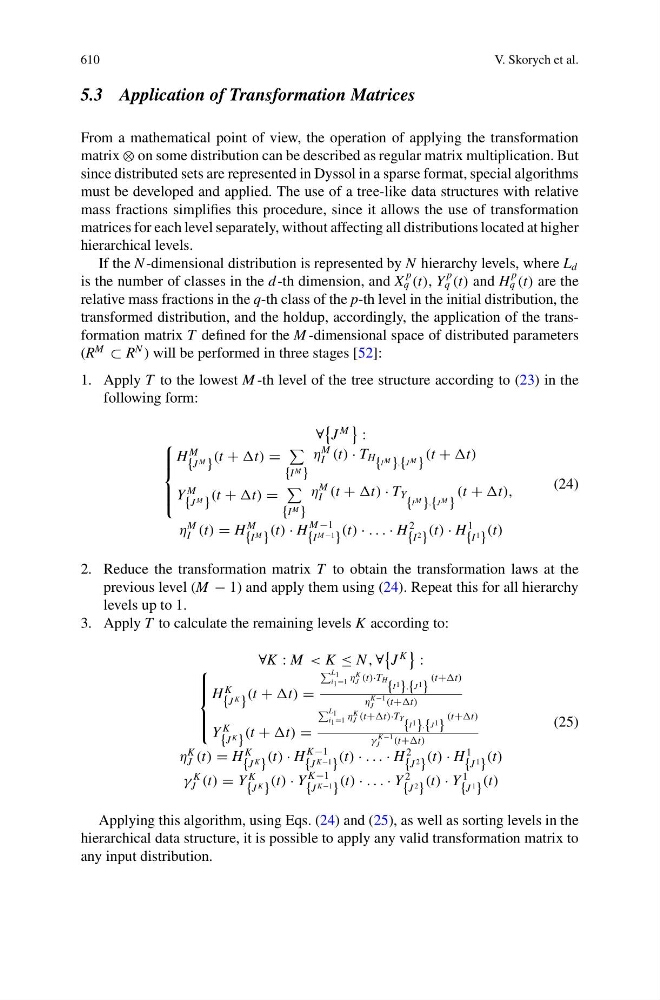
1. Apply T to the lowest M -th level of the tree structure according to (23) in the
following form:
∀
J
M
:
⎧
⎪ ⎪ ⎨
⎪ ⎪ ⎩
H
M
{J
M
} (t + t) =
{I
M
}
η
M
I (t) · T H { I M } , { J M }
(t + t)
Y
M
{J
M
} (t + t) =
{I
M
}
η
M
I (t + t) · T Y { I M } , { J M }
(t + t),
η
M
I (t) = H
M
{I
M
} (t) · H
M −1
{I
M −1
} (t) · . . . · H
2
{I
2
} (t) · H
1
{I
1
} (t)
(24)
2. Reduce the transformation matrix T to obtain the transformation laws at the
previous level (M − 1) and apply them using (24). Repeat this for all hierarchy
levels up to 1.
3. Apply T to calculate the remaining levels K according to:
∀K : M < K ≤ N , ∀
J
K
:
⎧
⎪ ⎪ ⎨
⎪ ⎪ ⎩
H
K
{J
K
} (t + t) =
L 1
i 1 =1 η
K
J (t)·TH { I 1 } , { J 1 }
(t+t)
η
K−1
J
(t+t)
Y
K
{J
K
} (t + t) =
L 1
i 1 =1 η
K
J (t+t)·TY { I 1 } , { J 1 }
(t+t)
γ
K−1
J
(t+t)
η
K
J (t) = H
K
{J
K
} (t) · H
K−1
{J
K−1
} (t) · . . . · H
2
{J
2
} (t) · H
1
{J
1
} (t)
γ
K
J (t) = Y
K
{J
K
} (t) · Y
K−1
{J
K−1
} (t) · . . . · Y
2
{J
2
} (t) · Y
1
{J
1
} (t)
(25)
Applying this algorithm, using Eqs. (24) and (25), as well as sorting levels in the
hierarchical data structure, it is possible to apply any valid transformation matrix to
any input distribution.
V. Skorych et al.
5.3 Application of Transformation Matrices
From a mathematical point of view, the operation of applying the transformation
matrix ⊗ on some distribution can be described as regular matrix multiplication. But
since distributed sets are represented in Dyssol in a sparse format, special algorithms
must be developed and applied. The use of a tree-like data structures with relative
mass fractions simplifies this procedure, since it allows the use of transformation
matrices for each level separately, without affecting all distributions located at higher
hierarchical levels.
If the N -dimensional distribution is represented by N hierarchy levels, where L d
is the number of classes in the d -th dimension, and X
p
q (t), Y
p
q (t) and H
p
q (t) are the
relative mass fractions in the q-th class of the p-th level in the initial distribution, the
transformed distribution, and the holdup, accordingly, the application of the transformation matrix T defined for the M -dimensional space of distributed parameters
(R
M
⊂ R
N ) will be performed in three stages [52]:
1. Apply T to the lowest M -th level of the tree structure according to (23) in the
following form:
∀
J
M
:
⎧
⎪ ⎪ ⎨
⎪ ⎪ ⎩
H
M
{J
M
} (t + t) =
{I
M
}
η
M
I (t) · T H { I M } , { J M }
(t + t)
Y
M
{J
M
} (t + t) =
{I
M
}
η
M
I (t + t) · T Y { I M } , { J M }
(t + t),
η
M
I (t) = H
M
{I
M
} (t) · H
M −1
{I
M −1
} (t) · . . . · H
2
{I
2
} (t) · H
1
{I
1
} (t)
(24)
2. Reduce the transformation matrix T to obtain the transformation laws at the
previous level (M − 1) and apply them using (24). Repeat this for all hierarchy
levels up to 1.
3. Apply T to calculate the remaining levels K according to:
∀K : M < K ≤ N , ∀
J
K
:
⎧
⎪ ⎪ ⎨
⎪ ⎪ ⎩
H
K
{J
K
} (t + t) =
L 1
i 1 =1 η
K
J (t)·TH { I 1 } , { J 1 }
(t+t)
η
K−1
J
(t+t)
Y
K
{J
K
} (t + t) =
L 1
i 1 =1 η
K
J (t+t)·TY { I 1 } , { J 1 }
(t+t)
γ
K−1
J
(t+t)
η
K
J (t) = H
K
{J
K
} (t) · H
K−1
{J
K−1
} (t) · . . . · H
2
{J
2
} (t) · H
1
{J
1
} (t)
γ
K
J (t) = Y
K
{J
K
} (t) · Y
K−1
{J
K−1
} (t) · . . . · Y
2
{J
2
} (t) · Y
1
{J
1
} (t)
(25)
Applying this algorithm, using Eqs. (24) and (25), as well as sorting levels in the
hierarchical data structure, it is possible to apply any valid transformation matrix to
any input distribution.