

17 A Framework for Dynamic Simulation of Interconnected …
589
the units and solvers are not directly integrated into the modelling system, but are
implemented as separate objects collected in the corresponding libraries. Herewith,
the set of available units and solvers can be expanded by each user, to allow for
modelling of specific problems.
New modules to be added to the modelling system can be developed using the
C++ programming language utilizing predefined programming interfaces. Therefore,
from a structural point of view, each unit is inherited from some basic object: base
unit or base solver (Fig. 4). On the one hand, these base objects provide new modules
with some primary functionality and give them access to other core and auxiliary
components. It allows them to treat material streams and holdups, to access compounds properties through materials database, to use interfaces to internal equation
solvers, to handle transformation matrices, etc. On the other hand, such basic modules define the interfaces via which the simulation system can interact with units and
solvers. In particular, each base object defines a certain set of functions that must be
extended by the developer of the model to implement the calculation algorithm of
individual unit or solver. These functions are run by the simulation system during
the execution of the main calculation algorithm. Both dynamic and steady-state units
can be developed using the provided interfaces.
The difference between solvers and units is that solvers are most often used not
directly by the simulation system, but by units to solve some sub-tasks within them.
Moreover, it becomes possible to implement several different solvers for a single task
of a certain type, and use them interchangeably within a unit. As an example, various
approaches to solving the population balance equations (PBE) for the agglomeration
process can be cited: using fixed pivot, cell average, or finite volume techniques—they
all can be used within a single agglomeration unit to handle the same problem.
To simplify the development of new modules, the Dyssol installation package
contains a Models creator kit with various templates of units and solvers, examples
and comprehensive documentation.
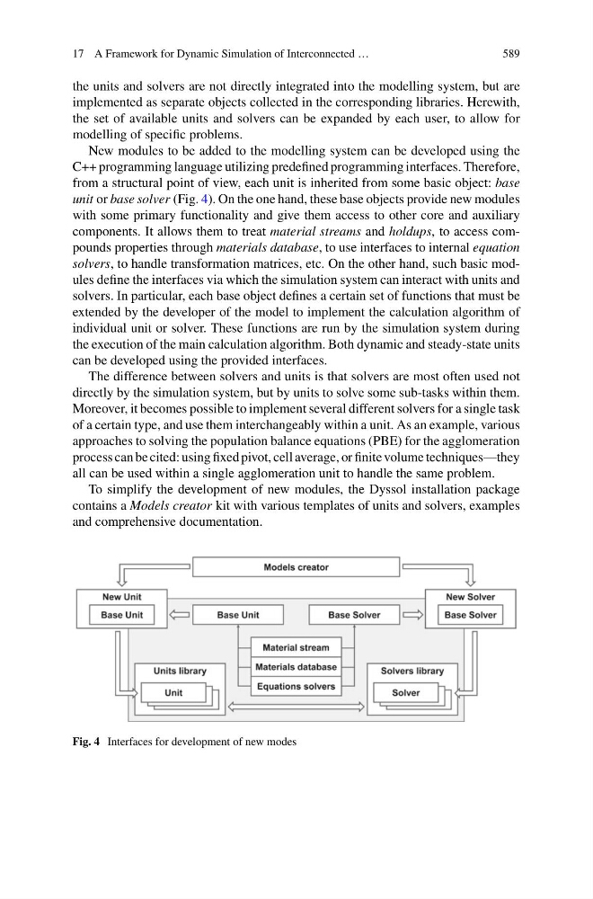
Fig. 4 Interfaces for development of new modes
589
the units and solvers are not directly integrated into the modelling system, but are
implemented as separate objects collected in the corresponding libraries. Herewith,
the set of available units and solvers can be expanded by each user, to allow for
modelling of specific problems.
New modules to be added to the modelling system can be developed using the
C++ programming language utilizing predefined programming interfaces. Therefore,
from a structural point of view, each unit is inherited from some basic object: base
unit or base solver (Fig. 4). On the one hand, these base objects provide new modules
with some primary functionality and give them access to other core and auxiliary
components. It allows them to treat material streams and holdups, to access compounds properties through materials database, to use interfaces to internal equation
solvers, to handle transformation matrices, etc. On the other hand, such basic modules define the interfaces via which the simulation system can interact with units and
solvers. In particular, each base object defines a certain set of functions that must be
extended by the developer of the model to implement the calculation algorithm of
individual unit or solver. These functions are run by the simulation system during
the execution of the main calculation algorithm. Both dynamic and steady-state units
can be developed using the provided interfaces.
The difference between solvers and units is that solvers are most often used not
directly by the simulation system, but by units to solve some sub-tasks within them.
Moreover, it becomes possible to implement several different solvers for a single task
of a certain type, and use them interchangeably within a unit. As an example, various
approaches to solving the population balance equations (PBE) for the agglomeration
process can be cited: using fixed pivot, cell average, or finite volume techniques—they
all can be used within a single agglomeration unit to handle the same problem.
To simplify the development of new modules, the Dyssol installation package
contains a Models creator kit with various templates of units and solvers, examples
and comprehensive documentation.
Fig. 4 Interfaces for development of new modes