

562
M. Spinola et al.
(a)
(b)
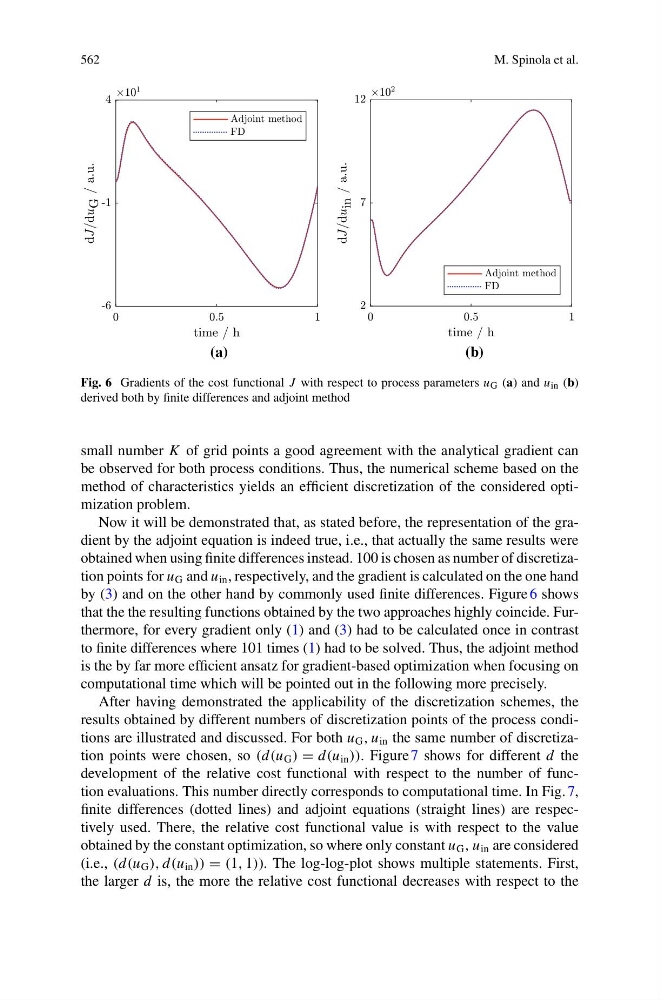
Fig. 6 Gradients of the cost functional J with respect to process parameters u G (a) and u in (b)
derived both by finite differences and adjoint method
small number K of grid points a good agreement with the analytical gradient can
be observed for both process conditions. Thus, the numerical scheme based on the
method of characteristics yields an efficient discretization of the considered optimization problem.
Now it will be demonstrated that, as stated before, the representation of the gradient by the adjoint equation is indeed true, i.e., that actually the same results were
obtained when using finite differences instead. 100 is chosen as number of discretization points for u G and u in , respectively, and the gradient is calculated on the one hand
by (3) and on the other hand by commonly used finite differences. Figure 6 shows
that the the resulting functions obtained by the two approaches highly coincide. Furthermore, for every gradient only (1) and (3) had to be calculated once in contrast
to finite differences where 101 times (1) had to be solved. Thus, the adjoint method
is the by far more efficient ansatz for gradient-based optimization when focusing on
computational time which will be pointed out in the following more precisely.
After having demonstrated the applicability of the discretization schemes, the
results obtained by different numbers of discretization points of the process conditions are illustrated and discussed. For both u G , u in the same number of discretization points were chosen, so (d(u G ) = d(u in )). Figure 7 shows for different d the
development of the relative cost functional with respect to the number of function evaluations. This number directly corresponds to computational time. In Fig. 7,
finite differences (dotted lines) and adjoint equations (straight lines) are respectively used. There, the relative cost functional value is with respect to the value
obtained by the constant optimization, so where only constant u G , u in are considered
(i.e., (d(u G ), d(u in )) = (1, 1)). The log-log-plot shows multiple statements. First,
the larger d is, the more the relative cost functional decreases with respect to the
M. Spinola et al.
(a)
(b)
Fig. 6 Gradients of the cost functional J with respect to process parameters u G (a) and u in (b)
derived both by finite differences and adjoint method
small number K of grid points a good agreement with the analytical gradient can
be observed for both process conditions. Thus, the numerical scheme based on the
method of characteristics yields an efficient discretization of the considered optimization problem.
Now it will be demonstrated that, as stated before, the representation of the gradient by the adjoint equation is indeed true, i.e., that actually the same results were
obtained when using finite differences instead. 100 is chosen as number of discretization points for u G and u in , respectively, and the gradient is calculated on the one hand
by (3) and on the other hand by commonly used finite differences. Figure 6 shows
that the the resulting functions obtained by the two approaches highly coincide. Furthermore, for every gradient only (1) and (3) had to be calculated once in contrast
to finite differences where 101 times (1) had to be solved. Thus, the adjoint method
is the by far more efficient ansatz for gradient-based optimization when focusing on
computational time which will be pointed out in the following more precisely.
After having demonstrated the applicability of the discretization schemes, the
results obtained by different numbers of discretization points of the process conditions are illustrated and discussed. For both u G , u in the same number of discretization points were chosen, so (d(u G ) = d(u in )). Figure 7 shows for different d the
development of the relative cost functional with respect to the number of function evaluations. This number directly corresponds to computational time. In Fig. 7,
finite differences (dotted lines) and adjoint equations (straight lines) are respectively used. There, the relative cost functional value is with respect to the value
obtained by the constant optimization, so where only constant u G , u in are considered
(i.e., (d(u G ), d(u in )) = (1, 1)). The log-log-plot shows multiple statements. First,
the larger d is, the more the relative cost functional decreases with respect to the