

16 Modeling, Simulation and Optimization of Process Chains
561
After having formulated the mathematical setting, the numerical results for this will
be focused in the following. In order to obtain a convenient graphical illustration of the
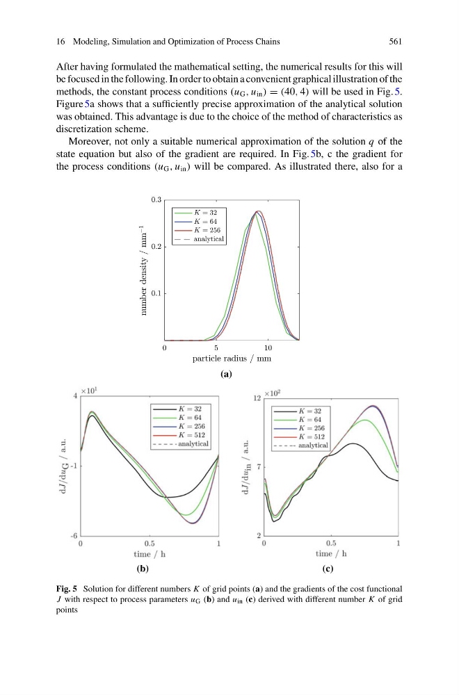
methods, the constant process conditions (u G , u in ) = (40, 4) will be used in Fig. 5.
Figure 5a shows that a sufficiently precise approximation of the analytical solution
was obtained. This advantage is due to the choice of the method of characteristics as
discretization scheme.
Moreover, not only a suitable numerical approximation of the solution q of the
state equation but also of the gradient are required. In Fig. 5b, c the gradient for
the process conditions (u G , u in ) will be compared. As illustrated there, also for a
Fig. 5 Solution for different numbers K of grid points (a) and the gradients of the cost functional
J with respect to process parameters u G (b) and u in (c) derived with different number K of grid
points
561
After having formulated the mathematical setting, the numerical results for this will
be focused in the following. In order to obtain a convenient graphical illustration of the
methods, the constant process conditions (u G , u in ) = (40, 4) will be used in Fig. 5.
Figure 5a shows that a sufficiently precise approximation of the analytical solution
was obtained. This advantage is due to the choice of the method of characteristics as
discretization scheme.
Moreover, not only a suitable numerical approximation of the solution q of the
state equation but also of the gradient are required. In Fig. 5b, c the gradient for
the process conditions (u G , u in ) will be compared. As illustrated there, also for a
Fig. 5 Solution for different numbers K of grid points (a) and the gradients of the cost functional
J with respect to process parameters u G (b) and u in (c) derived with different number K of grid
points