

560
M. Spinola et al.
4 Numerical Study
In this section, the outlined scheme for gradient approximation will be applied on
four examples. There synthesis processes and optimization goals are altered and
corresponding numerical results are shown. The first two deal with reaching desired
monomodal and bimodal PSDs, respectively, in a FBSG-like system. The third one
aims to obtain a monodisperse PSD in an Ostwald ripening like module. Eventually,
the last example considers a cycled process chain containing a FBSG-like module and
milling module. Furthermore, it has to be mentioned that even though the processes
in Sects. 4.3 and 4.4 cannot directly be represented by (1), the model can also be
extended to include these cases. For sake of a clearer illustration of the concepts, the
already stated (1) was chosen as the model depicting seeded growth processes. At
specific points, it is necessary to distinguish between the development of a PSD on a
whole time horizon and the corresponding PSD at a certain point in time. Thus, for
sake of a more precise notation, the “dot notation” will be introduced: If q denotes
the evolution of a PSD over [0, t f ], the underlying PSD at time t of q is denoted by
q(t, ·).
4.1 Fluidized Bed Spray Granulation: Reaching Desired
Monomodal PSDs
In this example, the underlying growth dynamics is chosen as it is typical for FBSG
(cf. [19]). Here, u G denotes the effective solid mass flux for the granulation process
that can be continuously adjusted. It is assumed that external nuclei with PSD q in
flow into the system over time by the rate u in . In the following, the relative standard
deviation (RSD) of a PSD is needed. The RSD is defined as
σ
μ
with the standard
deviation σ and mean particle size μ of a given PSD. Here, q in has a mean radius of
2 mm and a RSD of 10 %. Considering the process on the time interval [0, t f ] with
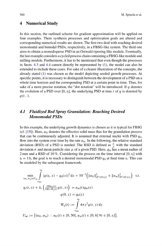
t f = 1 h, the goal is to reach a desired monomodal PSD q d at final time t f . This can
be modeled by the subsequent framework:
min
(u G ,u in )∈U ad
∞
x min
|q(t f , x) − q d (x)|
2 dx + 10
−3
u G
2
H 1 ((0,t f )) + +u in
2
H 1 ((0,t f ))
s.t.
q t (t, x) + ∂ x
100u G (t)
100+W q (t)
q(t, x)
= u in (t)q in (x)
q(0, x) = q 0 (x)
W q (t) :=
∞
x min
4π y
2 q(t, y) dy
U ad :=
(u G , u in ) : u G (t) ∈ [0, 50], u in (t) ∈ [0, 6] ∀t ∈ [0, t f ]
.
M. Spinola et al.
4 Numerical Study
In this section, the outlined scheme for gradient approximation will be applied on
four examples. There synthesis processes and optimization goals are altered and
corresponding numerical results are shown. The first two deal with reaching desired
monomodal and bimodal PSDs, respectively, in a FBSG-like system. The third one
aims to obtain a monodisperse PSD in an Ostwald ripening like module. Eventually,
the last example considers a cycled process chain containing a FBSG-like module and
milling module. Furthermore, it has to be mentioned that even though the processes
in Sects. 4.3 and 4.4 cannot directly be represented by (1), the model can also be
extended to include these cases. For sake of a clearer illustration of the concepts, the
already stated (1) was chosen as the model depicting seeded growth processes. At
specific points, it is necessary to distinguish between the development of a PSD on a
whole time horizon and the corresponding PSD at a certain point in time. Thus, for
sake of a more precise notation, the “dot notation” will be introduced: If q denotes
the evolution of a PSD over [0, t f ], the underlying PSD at time t of q is denoted by
q(t, ·).
4.1 Fluidized Bed Spray Granulation: Reaching Desired
Monomodal PSDs
In this example, the underlying growth dynamics is chosen as it is typical for FBSG
(cf. [19]). Here, u G denotes the effective solid mass flux for the granulation process
that can be continuously adjusted. It is assumed that external nuclei with PSD q in
flow into the system over time by the rate u in . In the following, the relative standard
deviation (RSD) of a PSD is needed. The RSD is defined as
σ
μ
with the standard
deviation σ and mean particle size μ of a given PSD. Here, q in has a mean radius of
2 mm and a RSD of 10 %. Considering the process on the time interval [0, t f ] with
t f = 1 h, the goal is to reach a desired monomodal PSD q d at final time t f . This can
be modeled by the subsequent framework:
min
(u G ,u in )∈U ad
∞
x min
|q(t f , x) − q d (x)|
2 dx + 10
−3
u G
2
H 1 ((0,t f )) + +u in
2
H 1 ((0,t f ))
s.t.
q t (t, x) + ∂ x
100u G (t)
100+W q (t)
q(t, x)
= u in (t)q in (x)
q(0, x) = q 0 (x)
W q (t) :=
∞
x min
4π y
2 q(t, y) dy
U ad :=
(u G , u in ) : u G (t) ∈ [0, 50], u in (t) ∈ [0, 6] ∀t ∈ [0, t f ]
.