

16 Modeling, Simulation and Optimization of Process Chains
559
ˆ
p k (t) = ˆ
p k (t f ) +
t f
t
J q [ ˆ
q, ˆ
q(t f , ·)](s, ˆ
ξ k (s)) + γ ( ˆ
ξ k (s))χ ( ˆ
ξ k (s)) ˆ
Y p (s) ds
−
t f
t
u out (s) ˆ
p k (s) ds
ˆ
Y p (t) =
K −1
k=1
1
2
q k−1 (t)( ˆ
p k−1 (t)+ ˆ
p k (t))
ˆ
ξ k (t)− ˆ
ξ k−1 (t)
+
q k (t)( ˆ
p k (t)+ ˆ
p k+1 (t))
ˆ
ξ k+1 (t)− ˆ
ξ k (t)
G W q
u G (t), ˆ
W q (t), t, ˆ
ξ k (t)
Where additionally it has to be set:
ˆ
p 0 := ˆ
p 1 ,
ˆ
p K +1 := ˆ
p K ,
ˆ
q 0 := 0,
ˆ
ξ 0 < ˆ
ξ 1 .
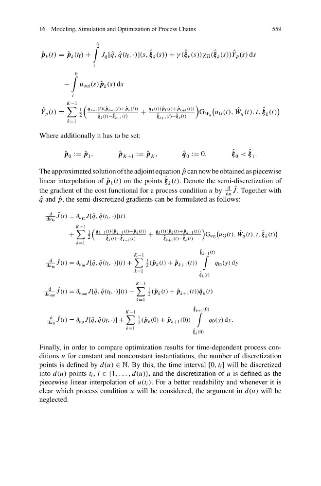
The approximated solution of the adjoint equation ˆ
p can now be obtained as piecewise
linear interpolation of ˆ
p k (t) on the points ˆ
ξ k (t). Denote the semi-discretization of
the gradient of the cost functional for a process condition u by
d
du
ˆ
J . Together with
ˆ
q and ˆ
p, the semi-discretized gradients can be formulated as follows:
d
du G
ˆ
J (t) = ∂ u G J [ ˆ
q, ˆ
q(t f , ·)](t)
+
K −1
k=1
1
2
q k−1 (t)( ˆ
p k−1 (t)+ ˆ
p k (t))
ˆ
ξ k (t)− ˆ
ξ k−1 (t)
+
q k (t)( ˆ
p k (t)+ ˆ
p k+1 (t))
ˆ
ξ k+1 (t)− ˆ
ξ k (t)
G u G
u G (t), ˆ
W q (t), t, ˆ
ξ k (t)
d
du in
ˆ
J (t) = ∂ u in J [ ˆ
q, ˆ
q(t f , ·)](t) +
K −1
k=1
1
2 ( ˆ
p k (t) + ˆ
p k+1 (t))
ˆ
ξ k+1 (t)
ˆ
ξ k (t)
q in (y) dy
d
du out
ˆ
J (t) = ∂ u out J [ ˆ
q, ˆ
q(t f , ·)](t) −
K −1
k=1
1
2 ( ˆ
p k (t) + ˆ
p k+1 (t)) ˆ
q k (t)
d
du 0
ˆ
J (t) = ∂ u 0 J [ ˆ
q, ˆ
q(t f , ·)] +
K −1
k=1
1
2 ( ˆ
p k (0) + ˆ
p k+1 (0))
ˆ
ξ k+1 (0)
ˆ
ξ k (0)
q 0 (y) dy.
Finally, in order to compare optimization results for time-dependent process conditions u for constant and nonconstant instantiations, the number of discretization
points is defined by d(u) ∈ N. By this, the time interval [0, t f ] will be discretized
into d(u) points t i , i ∈ {1, . . . , d(u)}, and the discretization of u is defined as the
piecewise linear interpolation of u(t i ). For a better readability and whenever it is
clear which process condition u will be considered, the argument in d(u) will be
neglected.
559
ˆ
p k (t) = ˆ
p k (t f ) +
t f
t
J q [ ˆ
q, ˆ
q(t f , ·)](s, ˆ
ξ k (s)) + γ ( ˆ
ξ k (s))χ ( ˆ
ξ k (s)) ˆ
Y p (s) ds
−
t f
t
u out (s) ˆ
p k (s) ds
ˆ
Y p (t) =
K −1
k=1
1
2
q k−1 (t)( ˆ
p k−1 (t)+ ˆ
p k (t))
ˆ
ξ k (t)− ˆ
ξ k−1 (t)
+
q k (t)( ˆ
p k (t)+ ˆ
p k+1 (t))
ˆ
ξ k+1 (t)− ˆ
ξ k (t)
G W q
u G (t), ˆ
W q (t), t, ˆ
ξ k (t)
Where additionally it has to be set:
ˆ
p 0 := ˆ
p 1 ,
ˆ
p K +1 := ˆ
p K ,
ˆ
q 0 := 0,
ˆ
ξ 0 < ˆ
ξ 1 .
The approximated solution of the adjoint equation ˆ
p can now be obtained as piecewise
linear interpolation of ˆ
p k (t) on the points ˆ
ξ k (t). Denote the semi-discretization of
the gradient of the cost functional for a process condition u by
d
du
ˆ
J . Together with
ˆ
q and ˆ
p, the semi-discretized gradients can be formulated as follows:
d
du G
ˆ
J (t) = ∂ u G J [ ˆ
q, ˆ
q(t f , ·)](t)
+
K −1
k=1
1
2
q k−1 (t)( ˆ
p k−1 (t)+ ˆ
p k (t))
ˆ
ξ k (t)− ˆ
ξ k−1 (t)
+
q k (t)( ˆ
p k (t)+ ˆ
p k+1 (t))
ˆ
ξ k+1 (t)− ˆ
ξ k (t)
G u G
u G (t), ˆ
W q (t), t, ˆ
ξ k (t)
d
du in
ˆ
J (t) = ∂ u in J [ ˆ
q, ˆ
q(t f , ·)](t) +
K −1
k=1
1
2 ( ˆ
p k (t) + ˆ
p k+1 (t))
ˆ
ξ k+1 (t)
ˆ
ξ k (t)
q in (y) dy
d
du out
ˆ
J (t) = ∂ u out J [ ˆ
q, ˆ
q(t f , ·)](t) −
K −1
k=1
1
2 ( ˆ
p k (t) + ˆ
p k+1 (t)) ˆ
q k (t)
d
du 0
ˆ
J (t) = ∂ u 0 J [ ˆ
q, ˆ
q(t f , ·)] +
K −1
k=1
1
2 ( ˆ
p k (0) + ˆ
p k+1 (0))
ˆ
ξ k+1 (0)
ˆ
ξ k (0)
q 0 (y) dy.
Finally, in order to compare optimization results for time-dependent process conditions u for constant and nonconstant instantiations, the number of discretization
points is defined by d(u) ∈ N. By this, the time interval [0, t f ] will be discretized
into d(u) points t i , i ∈ {1, . . . , d(u)}, and the discretization of u is defined as the
piecewise linear interpolation of u(t i ). For a better readability and whenever it is
clear which process condition u will be considered, the argument in d(u) will be
neglected.