

558
M. Spinola et al.
˙ ˆ
ξ k (t) = G(u G (t), ˆ
W q (t), t, ˆ
ξ k (τ ))
k ∈ {1, . . . , K }
˙
q k (t) := u in (t)
ˆ
ξ k+1 (t)
ˆ
ξ k (t)
q in (y) dy − u out (t)q k (t)
k ∈ {1, . . . , K − 1}
ˆ
W q (t) :=
K −1
k=1
q k (t)
ˆ
ξ k+1 (t)− ˆ
ξ k (t)
∞
x min
γ (y)χ ( ˆ
ξ k (t), ˆ
ξ k+1 (t)) (y) dy
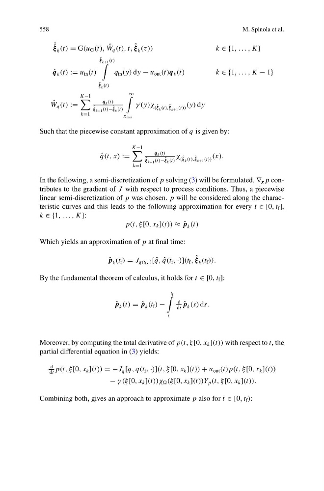
Such that the piecewise constant approximation of q is given by:
ˆ
q(t, x) :=
K −1
k=1
q k (t)
ˆ
ξ k+1 (t)− ˆ
ξ k (t)
χ ( ˆ
ξ k (t), ˆ
ξ k+1 (t)) (x).
In the following, a semi-discretization of p solving (3) will be formulated. ∇ x p contributes to the gradient of J with respect to process conditions. Thus, a piecewise
linear semi-discretization of p was chosen. p will be considered along the characteristic curves and this leads to the following approximation for every t ∈ [0, t f ],
k ∈ {1, . . . , K }:
p(t, ξ[0, x k ](t)) ≈ ˆ
p k (t)
Which yields an approximation of p at final time:
ˆ
p k (t f ) = J q(t f ,·) [ ˆ
q, ˆ
q(t f , ·)](t f , ˆ
ξ k (t f )).
By the fundamental theorem of calculus, it holds for t ∈ [0, t f ]:
ˆ
p k (t) = ˆ
p k (t f ) −
t f
t
d
dt
ˆ
p k (s) ds.
Moreover, by computing the total derivative of p(t, ξ[0, x k ](t)) with respect to t, the
partial differential equation in (3) yields:
d
dt
p(t, ξ[0, x k ](t)) = −J q [q, q(t f , ·)](t, ξ[0, x k ](t)) + u out (t) p(t, ξ[0, x k ](t))
− γ (ξ[0, x k ](t))χ (ξ [0, x k ](t))Y p (t, ξ[0, x k ](t)).
Combining both, gives an approach to approximate p also for t ∈ [0, t f ):
M. Spinola et al.
˙ ˆ
ξ k (t) = G(u G (t), ˆ
W q (t), t, ˆ
ξ k (τ ))
k ∈ {1, . . . , K }
˙
q k (t) := u in (t)
ˆ
ξ k+1 (t)
ˆ
ξ k (t)
q in (y) dy − u out (t)q k (t)
k ∈ {1, . . . , K − 1}
ˆ
W q (t) :=
K −1
k=1
q k (t)
ˆ
ξ k+1 (t)− ˆ
ξ k (t)
∞
x min
γ (y)χ ( ˆ
ξ k (t), ˆ
ξ k+1 (t)) (y) dy
Such that the piecewise constant approximation of q is given by:
ˆ
q(t, x) :=
K −1
k=1
q k (t)
ˆ
ξ k+1 (t)− ˆ
ξ k (t)
χ ( ˆ
ξ k (t), ˆ
ξ k+1 (t)) (x).
In the following, a semi-discretization of p solving (3) will be formulated. ∇ x p contributes to the gradient of J with respect to process conditions. Thus, a piecewise
linear semi-discretization of p was chosen. p will be considered along the characteristic curves and this leads to the following approximation for every t ∈ [0, t f ],
k ∈ {1, . . . , K }:
p(t, ξ[0, x k ](t)) ≈ ˆ
p k (t)
Which yields an approximation of p at final time:
ˆ
p k (t f ) = J q(t f ,·) [ ˆ
q, ˆ
q(t f , ·)](t f , ˆ
ξ k (t f )).
By the fundamental theorem of calculus, it holds for t ∈ [0, t f ]:
ˆ
p k (t) = ˆ
p k (t f ) −
t f
t
d
dt
ˆ
p k (s) ds.
Moreover, by computing the total derivative of p(t, ξ[0, x k ](t)) with respect to t, the
partial differential equation in (3) yields:
d
dt
p(t, ξ[0, x k ](t)) = −J q [q, q(t f , ·)](t, ξ[0, x k ](t)) + u out (t) p(t, ξ[0, x k ](t))
− γ (ξ[0, x k ](t))χ (ξ [0, x k ](t))Y p (t, ξ[0, x k ](t)).
Combining both, gives an approach to approximate p also for t ∈ [0, t f ):