

16 Modeling, Simulation and Optimization of Process Chains
557
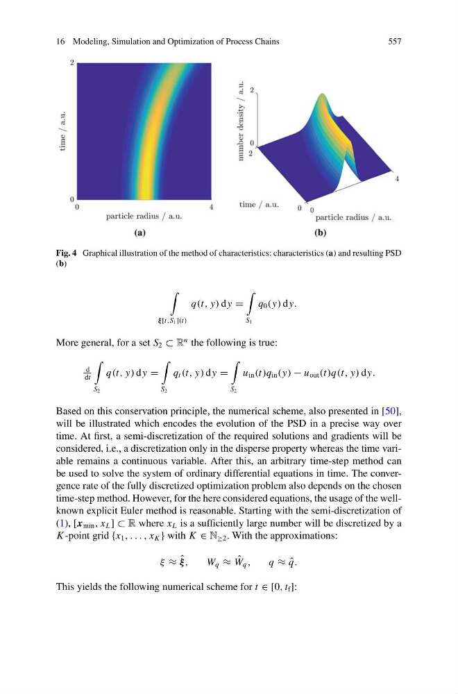
Fig. 4 Graphical illustration of the method of characteristics: characteristics (a) and resulting PSD
(b)
ξ [t,S 1 ](t)
q(t, y) dy =
S 1
q 0 (y) dy.
More general, for a set S 2 ⊂ R
n the following is true:
d
dt
S 2
q(t, y) dy =
S 2
q t (t, y) dy =
S 2
u in (t)q in (y) − u out (t)q(t, y) dy.
Based on this conservation principle, the numerical scheme, also presented in [50],
will be illustrated which encodes the evolution of the PSD in a precise way over
time. At first, a semi-discretization of the required solutions and gradients will be
considered, i.e., a discretization only in the disperse property whereas the time variable remains a continuous variable. After this, an arbitrary time-step method can
be used to solve the system of ordinary differential equations in time. The convergence rate of the fully discretized optimization problem also depends on the chosen
time-step method. However, for the here considered equations, the usage of the wellknown explicit Euler method is reasonable. Starting with the semi-discretization of
(1), [x min , x L ] ⊂ R where x L is a sufficiently large number will be discretized by a
K -point grid {x 1 , . . . , x K } with K ∈ N ≥2 . With the approximations:
ξ ≈ ˆ
ξ ,
W q ≈ ˆ
W q ,
q ≈ ˆ
q.
This yields the following numerical scheme for t ∈ [0, t f ]:
557
Fig. 4 Graphical illustration of the method of characteristics: characteristics (a) and resulting PSD
(b)
ξ [t,S 1 ](t)
q(t, y) dy =
S 1
q 0 (y) dy.
More general, for a set S 2 ⊂ R
n the following is true:
d
dt
S 2
q(t, y) dy =
S 2
q t (t, y) dy =
S 2
u in (t)q in (y) − u out (t)q(t, y) dy.
Based on this conservation principle, the numerical scheme, also presented in [50],
will be illustrated which encodes the evolution of the PSD in a precise way over
time. At first, a semi-discretization of the required solutions and gradients will be
considered, i.e., a discretization only in the disperse property whereas the time variable remains a continuous variable. After this, an arbitrary time-step method can
be used to solve the system of ordinary differential equations in time. The convergence rate of the fully discretized optimization problem also depends on the chosen
time-step method. However, for the here considered equations, the usage of the wellknown explicit Euler method is reasonable. Starting with the semi-discretization of
(1), [x min , x L ] ⊂ R where x L is a sufficiently large number will be discretized by a
K -point grid {x 1 , . . . , x K } with K ∈ N ≥2 . With the approximations:
ξ ≈ ˆ
ξ ,
W q ≈ ˆ
W q ,
q ≈ ˆ
q.
This yields the following numerical scheme for t ∈ [0, t f ]: