

556
M. Spinola et al.
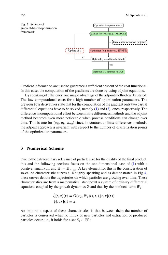
Fig. 3 Scheme of
gradient-based optimization
framework
Gradient information are used to guarantee a sufficient descent of the cost functional.
In this case, the computation of the gradients are done by using adjoint equations.
By speaking of efficiency, one major advantage of the adjoint method can be stated:
The low computational costs for a high number of optimization parameters. The
previous four derivatives state that for the computation of the gradient only two partial
differential equations have to be solved, namely (1) and (3), once, respectively. The
difference in computational effort between finite differences methods and the adjoint
method becomes even more noticeable when process conditions can change over
time. This is true for (u G , u in , u out ) since, in contrast to finite differences methods,
the adjoint approach is invariant with respect to the number of discretization points
of the optimization parameters.
3 Numerical Scheme
Due to the extraordinary relevance of particle size for the quality of the final product,
this and the following sections focus on the one-dimensional case of (1) with a
positive, small x min and := R >x min . A key element for this is the consideration of
so-called characteristic curves ξ . Roughly speaking and as demonstrated in Fig. 4,
these curves denote the trajectories on which particles are growing over time. These
characteristics are from a mathematical standpoint a system of ordinary differential
equations coupled by the growth dynamics G and thus by the nonlocal term W q :
˙
ξ [t, x](τ ) = G(u G , W q (t), t, ξ[t, x](τ ))
ξ [t, x](t) = x.
An important aspect of these characteristics is that between them the number of
particles is conserved when no influx of new particles and extraction of produced
particles occur, i.e., it holds for a set S 1 ⊂ R
n :
M. Spinola et al.
Fig. 3 Scheme of
gradient-based optimization
framework
Gradient information are used to guarantee a sufficient descent of the cost functional.
In this case, the computation of the gradients are done by using adjoint equations.
By speaking of efficiency, one major advantage of the adjoint method can be stated:
The low computational costs for a high number of optimization parameters. The
previous four derivatives state that for the computation of the gradient only two partial
differential equations have to be solved, namely (1) and (3), once, respectively. The
difference in computational effort between finite differences methods and the adjoint
method becomes even more noticeable when process conditions can change over
time. This is true for (u G , u in , u out ) since, in contrast to finite differences methods,
the adjoint approach is invariant with respect to the number of discretization points
of the optimization parameters.
3 Numerical Scheme
Due to the extraordinary relevance of particle size for the quality of the final product,
this and the following sections focus on the one-dimensional case of (1) with a
positive, small x min and := R >x min . A key element for this is the consideration of
so-called characteristic curves ξ . Roughly speaking and as demonstrated in Fig. 4,
these curves denote the trajectories on which particles are growing over time. These
characteristics are from a mathematical standpoint a system of ordinary differential
equations coupled by the growth dynamics G and thus by the nonlocal term W q :
˙
ξ [t, x](τ ) = G(u G , W q (t), t, ξ[t, x](τ ))
ξ [t, x](t) = x.
An important aspect of these characteristics is that between them the number of
particles is conserved when no influx of new particles and extraction of produced
particles occur, i.e., it holds for a set S 1 ⊂ R
n :