

16 Modeling, Simulation and Optimization of Process Chains
555
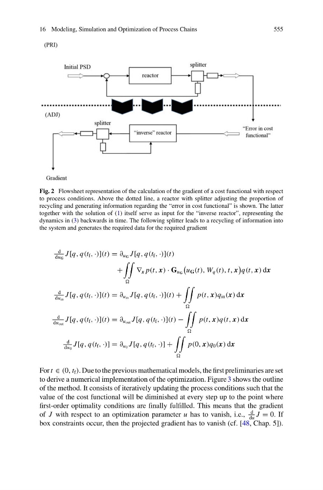
Fig. 2 Flowsheet representation of the calculation of the gradient of a cost functional with respect
to process conditions. Above the dotted line, a reactor with splitter adjusting the proportion of
recycling and generating information regarding the “error in cost functional” is shown. The latter
together with the solution of (1) itself serve as input for the “inverse reactor”, representing the
dynamics in (3) backwards in time. The following splitter leads to a recycling of information into
the system and generates the required data for the required gradient
d
du G
J [q, q(t f , ·)](t) = ∂ u G J [q, q(t f , ·)](t)
+
∇ x p(t, x) · G u G
u G (t), W q (t), t, x
q(t, x) dx
d
du in
J [q, q(t f , ·)](t) = ∂ u in J [q, q(t f , ·)](t) +
p(t, x)q in (x) dx
d
du out
J [q, q(t f , ·)](t) = ∂ u out J [q, q(t f , ·)](t) −
p(t, x)q(t, x) dx
d
du 0
J [q, q(t f , ·)] = ∂ u 0 J [q, q(t f , ·)] +
p(0, x)q 0 (x) dx
For t ∈ (0, t f ). Due to the previous mathematical models, the first preliminaries are set
to derive a numerical implementation of the optimization. Figure 3 shows the outline
of the method. It consists of iteratively updating the process conditions such that the
value of the cost functional will be diminished at every step up to the point where
first-order optimality conditions are finally fulfilled. This means that the gradient
of J with respect to an optimization parameter u has to vanish, i.e.,
d
du
J = 0. If
box constraints occur, then the projected gradient has to vanish (cf. [48, Chap. 5]).
555
Fig. 2 Flowsheet representation of the calculation of the gradient of a cost functional with respect
to process conditions. Above the dotted line, a reactor with splitter adjusting the proportion of
recycling and generating information regarding the “error in cost functional” is shown. The latter
together with the solution of (1) itself serve as input for the “inverse reactor”, representing the
dynamics in (3) backwards in time. The following splitter leads to a recycling of information into
the system and generates the required data for the required gradient
d
du G
J [q, q(t f , ·)](t) = ∂ u G J [q, q(t f , ·)](t)
+
∇ x p(t, x) · G u G
u G (t), W q (t), t, x
q(t, x) dx
d
du in
J [q, q(t f , ·)](t) = ∂ u in J [q, q(t f , ·)](t) +
p(t, x)q in (x) dx
d
du out
J [q, q(t f , ·)](t) = ∂ u out J [q, q(t f , ·)](t) −
p(t, x)q(t, x) dx
d
du 0
J [q, q(t f , ·)] = ∂ u 0 J [q, q(t f , ·)] +
p(0, x)q 0 (x) dx
For t ∈ (0, t f ). Due to the previous mathematical models, the first preliminaries are set
to derive a numerical implementation of the optimization. Figure 3 shows the outline
of the method. It consists of iteratively updating the process conditions such that the
value of the cost functional will be diminished at every step up to the point where
first-order optimality conditions are finally fulfilled. This means that the gradient
of J with respect to an optimization parameter u has to vanish, i.e.,
d
du
J = 0. If
box constraints occur, then the projected gradient has to vanish (cf. [48, Chap. 5]).