

554
M. Spinola et al.
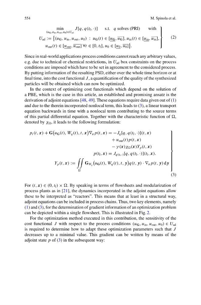
min
(u G ,u in ,u out ,u 0 )∈U ad
J [q, q(t f , ·)]
s.t. q solves (PRI)
with
U ad :=
(u G , u in , u out , u 0 ) : u G (t) ∈ [u G , u G ], u in (t) ∈ [u in , u in ],
u out (t) ∈ [u out , u out ] ∀t ∈ [0, t f ], u 0 ∈ [u 0 , u 0 ]
.
⎫
⎪ ⎪ ⎬
⎪ ⎪ ⎭
(2)
Since in real-world applications process conditions cannot reach any arbitrary values,
e.g. due to technical or chemical restrictions, in U ad box constraints on the process
conditions are imposed which have to be set in agreement to the considered process.
By putting information of the resulting PSD, either over the whole time horizon or at
final time, into the cost functional J , a quantification of the quality of the synthesized
particles will be obtained which can now be optimized.
In the context of optimizing cost functionals which depend on the solution of
a PBE, which is the case in this article, an established and promising ansatz is the
derivation of adjoint equations [48, 49]. These equations require data given out of (1)
and due to the therein incorporated nonlocal term, this leads to (3), a linear transport
equation backwards in time with a nonlocal term contributing to the source terms
of this partial differential equation. Together with the characteristic function of ,
denoted by χ , it leads to the following formulation:
p t (t, x) + G
u G (t), W q (t), t, x
∇ x p(t, x) = −J q [q, q(t f , ·)](t, x)
+ u out (t) p(t, x)
− γ (x)χ (x)Y p (t, x)
p(t f , x) = J q(t f ,·) [q, q(t f , ·)](t f , x).
Y p (t, x) :=
G W q
u G (t), W q (t), t, y
q(t, y) · ∇ x p(t, y) d y
⎫
⎪ ⎪ ⎪ ⎪ ⎪ ⎪ ⎪ ⎪ ⎪ ⎬
⎪ ⎪ ⎪ ⎪ ⎪ ⎪ ⎪ ⎪ ⎪ ⎭
(3)
For (t, x) ∈ (0, t f ) × . By speaking in terms of flowsheets and modularization of
process plants as in [21], the dynamics incorporated in the adjoint equations allow
these to be interpreted as “reactors”. This means that at least in a structural way,
adjoint equations can be included in process chains. Thus, two key elements, namely
(1) and (3), for the determination of gradient information of an optimization problem
can be depicted within a single flowsheet. This is illustrated in Fig. 2.
For the optimization method executed in this contribution, the sensitivity of the
cost functional J with respect to the process conditions (u G , u in , u out , u 0 ) ∈ U ad
is required to determine how to adapt these optimization parameters such that J
decreases up to a minimal value. This gradient can be written by means of the
adjoint state p of (3) in the subsequent way:
M. Spinola et al.
min
(u G ,u in ,u out ,u 0 )∈U ad
J [q, q(t f , ·)]
s.t. q solves (PRI)
with
U ad :=
(u G , u in , u out , u 0 ) : u G (t) ∈ [u G , u G ], u in (t) ∈ [u in , u in ],
u out (t) ∈ [u out , u out ] ∀t ∈ [0, t f ], u 0 ∈ [u 0 , u 0 ]
.
⎫
⎪ ⎪ ⎬
⎪ ⎪ ⎭
(2)
Since in real-world applications process conditions cannot reach any arbitrary values,
e.g. due to technical or chemical restrictions, in U ad box constraints on the process
conditions are imposed which have to be set in agreement to the considered process.
By putting information of the resulting PSD, either over the whole time horizon or at
final time, into the cost functional J , a quantification of the quality of the synthesized
particles will be obtained which can now be optimized.
In the context of optimizing cost functionals which depend on the solution of
a PBE, which is the case in this article, an established and promising ansatz is the
derivation of adjoint equations [48, 49]. These equations require data given out of (1)
and due to the therein incorporated nonlocal term, this leads to (3), a linear transport
equation backwards in time with a nonlocal term contributing to the source terms
of this partial differential equation. Together with the characteristic function of ,
denoted by χ , it leads to the following formulation:
p t (t, x) + G
u G (t), W q (t), t, x
∇ x p(t, x) = −J q [q, q(t f , ·)](t, x)
+ u out (t) p(t, x)
− γ (x)χ (x)Y p (t, x)
p(t f , x) = J q(t f ,·) [q, q(t f , ·)](t f , x).
Y p (t, x) :=
G W q
u G (t), W q (t), t, y
q(t, y) · ∇ x p(t, y) d y
⎫
⎪ ⎪ ⎪ ⎪ ⎪ ⎪ ⎪ ⎪ ⎪ ⎬
⎪ ⎪ ⎪ ⎪ ⎪ ⎪ ⎪ ⎪ ⎪ ⎭
(3)
For (t, x) ∈ (0, t f ) × . By speaking in terms of flowsheets and modularization of
process plants as in [21], the dynamics incorporated in the adjoint equations allow
these to be interpreted as “reactors”. This means that at least in a structural way,
adjoint equations can be included in process chains. Thus, two key elements, namely
(1) and (3), for the determination of gradient information of an optimization problem
can be depicted within a single flowsheet. This is illustrated in Fig. 2.
For the optimization method executed in this contribution, the sensitivity of the
cost functional J with respect to the process conditions (u G , u in , u out , u 0 ) ∈ U ad
is required to determine how to adapt these optimization parameters such that J
decreases up to a minimal value. This gradient can be written by means of the
adjoint state p of (3) in the subsequent way: