

16 Modeling, Simulation and Optimization of Process Chains
563
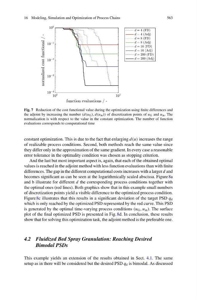
Fig. 7 Reduction of the cost functional value during the optimization using finite differences and
the adjoint by increasing the number (d(u G ), d(u in )) of discretization points of u G and u in . The
normalization is with respect to the value in the constant optimization. The number of function
evaluations corresponds to computational time
constant optimization. This is due to the fact that enlarging d(u) increases the range
of realizable process conditions. Second, both methods reach the same value since
they differ only in the approximation of the same gradient. In every case a reasonable
error tolerance in the optimality condition was chosen as stopping criterion.
And the last but most important aspect is, again, that each of the obtained optimal
values is reached in the adjoint method with less function evaluations than with finite
differences. The gap in the different computational costs increases with a larger d and
becomes significant as can be seen at the logarithmically scaled abscissa. Figure 8a
and b illustrate for different d the corresponding process conditions together with
the optimal ones (red lines). Both graphics show that in this example small numbers
of discretization points yield a visible difference to the optimized process condition.
Figure 8c illustrates that this results in a significant deviation of the target PSD q d
which is only reached by the optimized PSD represented by the red curve. This PSD
is generated by the optimal time-varying process conditions (u G , u in ). The surface
plot of the final optimized PSD is presented in Fig. 8d. In conclusion, these results
show that for solving this optimization task, the adjoint method is the preferable one.
4.2 Fluidized Bed Spray Granulation: Reaching Desired
Bimodal PSDs
This example yields an extension of the results obtained in Sect. 4.1. The same
setup as in there will be considered but the desired PSD q d is bimodal. As discussed
563
Fig. 7 Reduction of the cost functional value during the optimization using finite differences and
the adjoint by increasing the number (d(u G ), d(u in )) of discretization points of u G and u in . The
normalization is with respect to the value in the constant optimization. The number of function
evaluations corresponds to computational time
constant optimization. This is due to the fact that enlarging d(u) increases the range
of realizable process conditions. Second, both methods reach the same value since
they differ only in the approximation of the same gradient. In every case a reasonable
error tolerance in the optimality condition was chosen as stopping criterion.
And the last but most important aspect is, again, that each of the obtained optimal
values is reached in the adjoint method with less function evaluations than with finite
differences. The gap in the different computational costs increases with a larger d and
becomes significant as can be seen at the logarithmically scaled abscissa. Figure 8a
and b illustrate for different d the corresponding process conditions together with
the optimal ones (red lines). Both graphics show that in this example small numbers
of discretization points yield a visible difference to the optimized process condition.
Figure 8c illustrates that this results in a significant deviation of the target PSD q d
which is only reached by the optimized PSD represented by the red curve. This PSD
is generated by the optimal time-varying process conditions (u G , u in ). The surface
plot of the final optimized PSD is presented in Fig. 8d. In conclusion, these results
show that for solving this optimization task, the adjoint method is the preferable one.
4.2 Fluidized Bed Spray Granulation: Reaching Desired
Bimodal PSDs
This example yields an extension of the results obtained in Sect. 4.1. The same
setup as in there will be considered but the desired PSD q d is bimodal. As discussed