

512
R. Ahrens et al.
Setting κ agg (m, m
) = 1 eliminates the kernel from the equation. The domain of
integration of the inner integral in the source term can be expanded to [0, m max ]
2 by
setting f (m − m
) := 0 if any component of m − m
is negative. A further change
in the integration variable gives
dM e (f )(t)
dt
=
1
2
Ω int
Ω int
f (m)f (m
) · (m 1 + m
1 )
e 1 · (m 2 + m
2 )
e 2 d m
d m
−
Ω int
Ω int
m
e 1
1 m
e 2
2 f (m)f (m
) d m
d m.
The binomials in the first line are expanded in order to separate the integrations with
respect to m and m
and then the order of summations and integrations is changed.
A similar separation in the second line leads to
dM e (f )(t)
dt
=
1
2
e 1
k 1 =0
e 2
k 2 =0
e 1
k 1
e 2
k 2
Ω int
m
k f (m) d m ·
Ω int
m
e−k f (m
) d m
−
Ω int
m
e 1
1 m
e 2
2 f (m) d m ·
Ω int
f (m
) d m
.
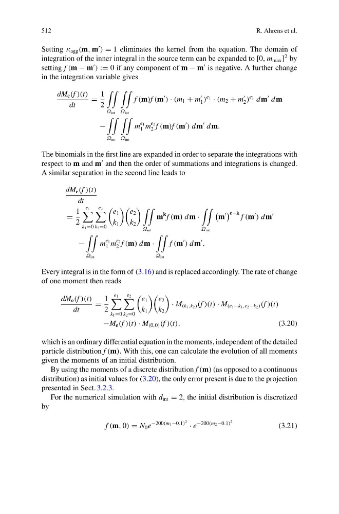
Every integral is in the form of (3.16) and is replaced accordingly. The rate of change
of one moment then reads
dM e (f )(t)
dt
=
1
2
e 1
k 1 =0
e 2
k 2 =0
e 1
k 1
e 2
k 2
· M (k 1 ,k 2 ) (f )(t) · M (e 1 −k 1 ,e 2 −k 2 ) (f )(t)
−M e (f )(t) · M (0,0) (f )(t),
(3.20)
which is an ordinary differential equation in the moments, independent of the detailed
particle distribution f (m). With this, one can calculate the evolution of all moments
given the moments of an initial distribution.
By using the moments of a discrete distribution f (m) (as opposed to a continuous
distribution) as initial values for (3.20), the only error present is due to the projection
presented in Sect. 3.2.3.
For the numerical simulation with d int = 2, the initial distribution is discretized
by
f (m, 0) = N 0 e
−200(m 1 −0.1)
2 · e
−200(m 2 −0.1)
2
(3.21)
R. Ahrens et al.
Setting κ agg (m, m
) = 1 eliminates the kernel from the equation. The domain of
integration of the inner integral in the source term can be expanded to [0, m max ]
2 by
setting f (m − m
) := 0 if any component of m − m
is negative. A further change
in the integration variable gives
dM e (f )(t)
dt
=
1
2
Ω int
Ω int
f (m)f (m
) · (m 1 + m
1 )
e 1 · (m 2 + m
2 )
e 2 d m
d m
−
Ω int
Ω int
m
e 1
1 m
e 2
2 f (m)f (m
) d m
d m.
The binomials in the first line are expanded in order to separate the integrations with
respect to m and m
and then the order of summations and integrations is changed.
A similar separation in the second line leads to
dM e (f )(t)
dt
=
1
2
e 1
k 1 =0
e 2
k 2 =0
e 1
k 1
e 2
k 2
Ω int
m
k f (m) d m ·
Ω int
m
e−k f (m
) d m
−
Ω int
m
e 1
1 m
e 2
2 f (m) d m ·
Ω int
f (m
) d m
.
Every integral is in the form of (3.16) and is replaced accordingly. The rate of change
of one moment then reads
dM e (f )(t)
dt
=
1
2
e 1
k 1 =0
e 2
k 2 =0
e 1
k 1
e 2
k 2
· M (k 1 ,k 2 ) (f )(t) · M (e 1 −k 1 ,e 2 −k 2 ) (f )(t)
−M e (f )(t) · M (0,0) (f )(t),
(3.20)
which is an ordinary differential equation in the moments, independent of the detailed
particle distribution f (m). With this, one can calculate the evolution of all moments
given the moments of an initial distribution.
By using the moments of a discrete distribution f (m) (as opposed to a continuous
distribution) as initial values for (3.20), the only error present is due to the projection
presented in Sect. 3.2.3.
For the numerical simulation with d int = 2, the initial distribution is discretized
by
f (m, 0) = N 0 e
−200(m 1 −0.1)
2 · e
−200(m 2 −0.1)
2
(3.21)