

14 Numerical Methods for Coupled Population Balance Systems …
511
M e (( j ) =
k={−1,0} d int
M e (C j+k )
⇐⇒ F j
d int
q=1
I
j q
e q =
k={−1,0} d int
w j+k
d int
q=1
J
j q +k q
e q
.
(3.19)
By using
J
j−1
e
+ J
j
e =
2h, if e = 0,
2h
2 j, if e = 1
= 2I
j
e ,
which follows directly from the definitions of (3.17) and (3.18), one pairs the 2
d int
summands in (3.19) and obtains
w j+k =
F j
2 d int
,
implying a uniform distribution of particles associated with a single grid-point g j to
its surrounding 2
d int cells.
This result is somewhat surprising as it does neither rely on the size of the grid
(the cell-width h) nor the index j of the cell in question. Further details can also be
found in [2].
3.2.4 Multi-variate Moments for the Pure Agglomeration Settings
This section is devoted to the analysis of moments M e (f )(t) of a multi-variate particle
distribution f (m) over time. For this, one obtains expressions to track any multivariate moment in the absence of breakage and growth and compares those values to
numerical moments obtained over the course of a simulation using the discretization
presented here.
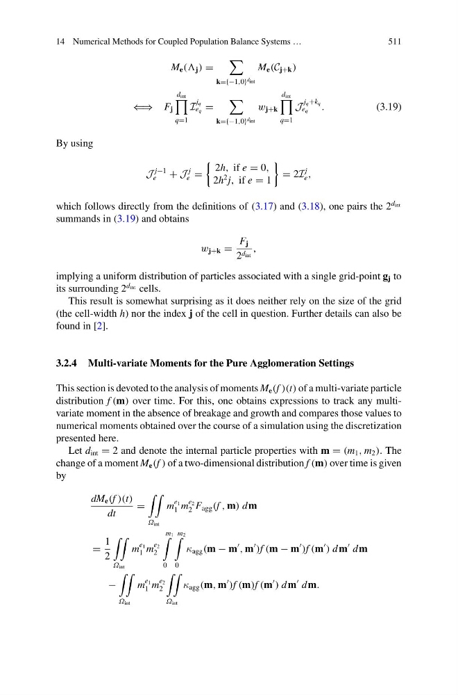
Let d int = 2 and denote the internal particle properties with m = (m 1 , m 2 ). The
change of a moment M e (f ) of a two-dimensional distribution f (m) over time is given
by
dM e (f )(t)
dt
=
Ω int
m
e 1
1 m
e 2
2 F agg (f , m) d m
=
1
2
Ω int
m
e 1
1 m
e 2
2
m 1
0
m 2
0
κ agg (m − m
, m
)f (m − m
)f (m
) d m
d m
−
Ω int
m
e 1
1 m
e 2
2
Ω int
κ agg (m, m
)f (m)f (m
) d m
d m.
511
M e (( j ) =
k={−1,0} d int
M e (C j+k )
⇐⇒ F j
d int
q=1
I
j q
e q =
k={−1,0} d int
w j+k
d int
q=1
J
j q +k q
e q
.
(3.19)
By using
J
j−1
e
+ J
j
e =
2h, if e = 0,
2h
2 j, if e = 1
= 2I
j
e ,
which follows directly from the definitions of (3.17) and (3.18), one pairs the 2
d int
summands in (3.19) and obtains
w j+k =
F j
2 d int
,
implying a uniform distribution of particles associated with a single grid-point g j to
its surrounding 2
d int cells.
This result is somewhat surprising as it does neither rely on the size of the grid
(the cell-width h) nor the index j of the cell in question. Further details can also be
found in [2].
3.2.4 Multi-variate Moments for the Pure Agglomeration Settings
This section is devoted to the analysis of moments M e (f )(t) of a multi-variate particle
distribution f (m) over time. For this, one obtains expressions to track any multivariate moment in the absence of breakage and growth and compares those values to
numerical moments obtained over the course of a simulation using the discretization
presented here.
Let d int = 2 and denote the internal particle properties with m = (m 1 , m 2 ). The
change of a moment M e (f ) of a two-dimensional distribution f (m) over time is given
by
dM e (f )(t)
dt
=
Ω int
m
e 1
1 m
e 2
2 F agg (f , m) d m
=
1
2
Ω int
m
e 1
1 m
e 2
2
m 1
0
m 2
0
κ agg (m − m
, m
)f (m − m
)f (m
) d m
d m
−
Ω int
m
e 1
1 m
e 2
2
Ω int
κ agg (m, m
)f (m)f (m
) d m
d m.