

14 Numerical Methods for Coupled Population Balance Systems …
513
0
1 0
2 0
3 0
4 0
5 0
t
0.98
0.99
1
1.01
1.02
A
(0,0)
Comparison of
(0,0)
(a)
0
1 0
2 0
3 0
4 0
5 0
t
0.98
0.99
1
1.01
1.02
A
(1,1)
Comparison of
(1,1)
(b)
0
1 0
2 0
3 0
4 0
5 0
t
0.98
0.99
1
1.01
1.02
A
(2,2)
Comparison of
(2,2)
(c)
0
1 0
2 0
3 0
4 0
5 0
t
0.98
0.99
1
1.01
1.02
A
(3,3)
Comparison of
(3,3)
(d)
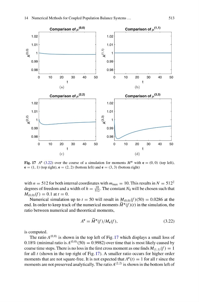
Fig. 17 A e (3.22) over the course of a simulation for moments M e with e = (0, 0) (top left),
e = (1, 1) (top right), e = (2, 2) (bottom left) and e = (3, 3) (bottom right)
with n = 512 for both internal coordinates with m max = 10. This results in N = 512
2
degrees of freedom and a width of h =
10
512
. The constant N 0 will be chosen such that
M (0,0) (f ) = 0.1 at t = 0.
Numerical simulation up to t = 50 will result in M (0,0) (f )(50) = 0.0286 at the
end. In order to keep track of the numerical moments
M
e
(f )(t) in the simulation, the
ratio between numerical and theoretical moments,
A
e
=
M
e
(f )/M e (f ),
(3.22)
is computed.
The ratio A
(0,0) is shown in the top left of Fig. 17 which displays a small loss of
0.18% (minimal ratio is A
(0,0)
(50) = 0.9982) over time that is most likely caused by
coarse time steps. There is no loss in the first cross moment as one finds M (1,1) (f ) = 1
for all t (shown in the top right of Fig. 17). A smaller ratio occurs for higher order
moments that are not square-free. It is not expected that A
e
(t) = 1 for all t since the
moments are not preserved analytically. The ratio A
(2,2) is shown in the bottom left of
513
0
1 0
2 0
3 0
4 0
5 0
t
0.98
0.99
1
1.01
1.02
A
(0,0)
Comparison of
(0,0)
(a)
0
1 0
2 0
3 0
4 0
5 0
t
0.98
0.99
1
1.01
1.02
A
(1,1)
Comparison of
(1,1)
(b)
0
1 0
2 0
3 0
4 0
5 0
t
0.98
0.99
1
1.01
1.02
A
(2,2)
Comparison of
(2,2)
(c)
0
1 0
2 0
3 0
4 0
5 0
t
0.98
0.99
1
1.01
1.02
A
(3,3)
Comparison of
(3,3)
(d)
Fig. 17 A e (3.22) over the course of a simulation for moments M e with e = (0, 0) (top left),
e = (1, 1) (top right), e = (2, 2) (bottom left) and e = (3, 3) (bottom right)
with n = 512 for both internal coordinates with m max = 10. This results in N = 512
2
degrees of freedom and a width of h =
10
512
. The constant N 0 will be chosen such that
M (0,0) (f ) = 0.1 at t = 0.
Numerical simulation up to t = 50 will result in M (0,0) (f )(50) = 0.0286 at the
end. In order to keep track of the numerical moments
M
e
(f )(t) in the simulation, the
ratio between numerical and theoretical moments,
A
e
=
M
e
(f )/M e (f ),
(3.22)
is computed.
The ratio A
(0,0) is shown in the top left of Fig. 17 which displays a small loss of
0.18% (minimal ratio is A
(0,0)
(50) = 0.9982) over time that is most likely caused by
coarse time steps. There is no loss in the first cross moment as one finds M (1,1) (f ) = 1
for all t (shown in the top right of Fig. 17). A smaller ratio occurs for higher order
moments that are not square-free. It is not expected that A
e
(t) = 1 for all t since the
moments are not preserved analytically. The ratio A
(2,2) is shown in the bottom left of