

13 Morphological Modelling and Simulation …
451
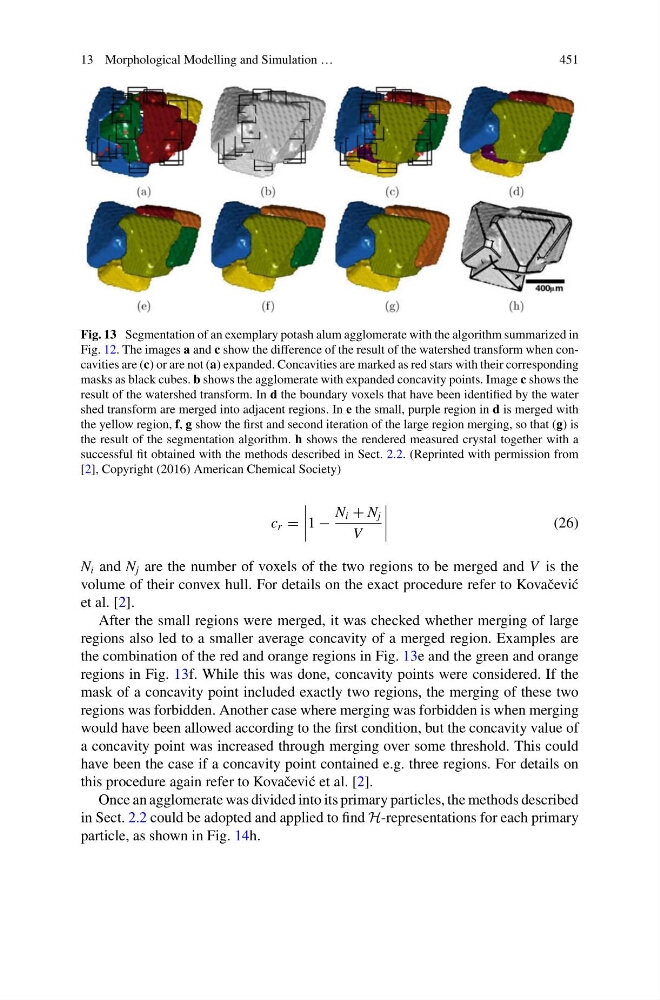
Fig. 13 Segmentation of an exemplary potash alum agglomerate with the algorithm summarized in
Fig. 12. The images a and c show the difference of the result of the watershed transform when concavities are (c) or are not (a) expanded. Concavities are marked as red stars with their corresponding
masks as black cubes. b shows the agglomerate with expanded concavity points. Image c shows the
result of the watershed transform. In d the boundary voxels that have been identified by the water
shed transform are merged into adjacent regions. In e the small, purple region in d is merged with
the yellow region, f, g show the first and second iteration of the large region merging, so that (g) is
the result of the segmentation algorithm. h shows the rendered measured crystal together with a
successful fit obtained with the methods described in Sect. 2.2. (Reprinted with permission from
[2], Copyright (2016) American Chemical Society)
c r =
1 −
N i + N j
V
(26)
N i and N j are the number of voxels of the two regions to be merged and V is the
volume of their convex hull. For details on the exact procedure refer to Kovaˇ cevi´ c
et al. [2].
After the small regions were merged, it was checked whether merging of large
regions also led to a smaller average concavity of a merged region. Examples are
the combination of the red and orange regions in Fig. 13e and the green and orange
regions in Fig. 13f. While this was done, concavity points were considered. If the
mask of a concavity point included exactly two regions, the merging of these two
regions was forbidden. Another case where merging was forbidden is when merging
would have been allowed according to the first condition, but the concavity value of
a concavity point was increased through merging over some threshold. This could
have been the case if a concavity point contained e.g. three regions. For details on
this procedure again refer to Kovaˇ cevi´ c et al. [2].
Once an agglomerate was divided into its primary particles, the methods described
in Sect. 2.2 could be adopted and applied to find H-representations for each primary
particle, as shown in Fig. 14h.
451
Fig. 13 Segmentation of an exemplary potash alum agglomerate with the algorithm summarized in
Fig. 12. The images a and c show the difference of the result of the watershed transform when concavities are (c) or are not (a) expanded. Concavities are marked as red stars with their corresponding
masks as black cubes. b shows the agglomerate with expanded concavity points. Image c shows the
result of the watershed transform. In d the boundary voxels that have been identified by the water
shed transform are merged into adjacent regions. In e the small, purple region in d is merged with
the yellow region, f, g show the first and second iteration of the large region merging, so that (g) is
the result of the segmentation algorithm. h shows the rendered measured crystal together with a
successful fit obtained with the methods described in Sect. 2.2. (Reprinted with permission from
[2], Copyright (2016) American Chemical Society)
c r =
1 −
N i + N j
V
(26)
N i and N j are the number of voxels of the two regions to be merged and V is the
volume of their convex hull. For details on the exact procedure refer to Kovaˇ cevi´ c
et al. [2].
After the small regions were merged, it was checked whether merging of large
regions also led to a smaller average concavity of a merged region. Examples are
the combination of the red and orange regions in Fig. 13e and the green and orange
regions in Fig. 13f. While this was done, concavity points were considered. If the
mask of a concavity point included exactly two regions, the merging of these two
regions was forbidden. Another case where merging was forbidden is when merging
would have been allowed according to the first condition, but the concavity value of
a concavity point was increased through merging over some threshold. This could
have been the case if a concavity point contained e.g. three regions. For details on
this procedure again refer to Kovaˇ cevi´ c et al. [2].
Once an agglomerate was divided into its primary particles, the methods described
in Sect. 2.2 could be adopted and applied to find H-representations for each primary
particle, as shown in Fig. 14h.