

452
S. Schiele et al.
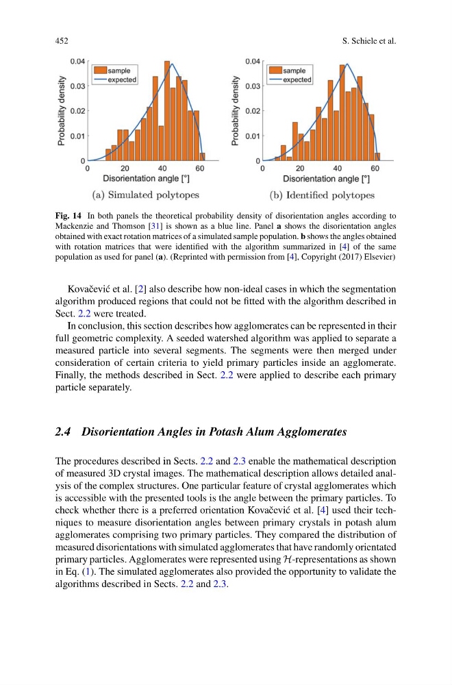
Fig. 14 In both panels the theoretical probability density of disorientation angles according to
Mackenzie and Thomson [31] is shown as a blue line. Panel a shows the disorientation angles
obtained with exact rotation matrices of a simulated sample population. b shows the angles obtained
with rotation matrices that were identified with the algorithm summarized in [4] of the same
population as used for panel (a). (Reprinted with permission from [4], Copyright (2017) Elsevier)
Kovaˇ cevi´ c et al. [2] also describe how non-ideal cases in which the segmentation
algorithm produced regions that could not be fitted with the algorithm described in
Sect. 2.2 were treated.
In conclusion, this section describes how agglomerates can be represented in their
full geometric complexity. A seeded watershed algorithm was applied to separate a
measured particle into several segments. The segments were then merged under
consideration of certain criteria to yield primary particles inside an agglomerate.
Finally, the methods described in Sect. 2.2 were applied to describe each primary
particle separately.
2.4 Disorientation Angles in Potash Alum Agglomerates
The procedures described in Sects. 2.2 and 2.3 enable the mathematical description
of measured 3D crystal images. The mathematical description allows detailed analysis of the complex structures. One particular feature of crystal agglomerates which
is accessible with the presented tools is the angle between the primary particles. To
check whether there is a preferred orientation Kovaˇ cevi´ c et al. [4] used their techniques to measure disorientation angles between primary crystals in potash alum
agglomerates comprising two primary particles. They compared the distribution of
measured disorientations with simulated agglomerates that have randomly orientated
primary particles. Agglomerates were represented using H-representations as shown
in Eq. (1). The simulated agglomerates also provided the opportunity to validate the
algorithms described in Sects. 2.2 and 2.3.
S. Schiele et al.
Fig. 14 In both panels the theoretical probability density of disorientation angles according to
Mackenzie and Thomson [31] is shown as a blue line. Panel a shows the disorientation angles
obtained with exact rotation matrices of a simulated sample population. b shows the angles obtained
with rotation matrices that were identified with the algorithm summarized in [4] of the same
population as used for panel (a). (Reprinted with permission from [4], Copyright (2017) Elsevier)
Kovaˇ cevi´ c et al. [2] also describe how non-ideal cases in which the segmentation
algorithm produced regions that could not be fitted with the algorithm described in
Sect. 2.2 were treated.
In conclusion, this section describes how agglomerates can be represented in their
full geometric complexity. A seeded watershed algorithm was applied to separate a
measured particle into several segments. The segments were then merged under
consideration of certain criteria to yield primary particles inside an agglomerate.
Finally, the methods described in Sect. 2.2 were applied to describe each primary
particle separately.
2.4 Disorientation Angles in Potash Alum Agglomerates
The procedures described in Sects. 2.2 and 2.3 enable the mathematical description
of measured 3D crystal images. The mathematical description allows detailed analysis of the complex structures. One particular feature of crystal agglomerates which
is accessible with the presented tools is the angle between the primary particles. To
check whether there is a preferred orientation Kovaˇ cevi´ c et al. [4] used their techniques to measure disorientation angles between primary crystals in potash alum
agglomerates comprising two primary particles. They compared the distribution of
measured disorientations with simulated agglomerates that have randomly orientated
primary particles. Agglomerates were represented using H-representations as shown
in Eq. (1). The simulated agglomerates also provided the opportunity to validate the
algorithms described in Sects. 2.2 and 2.3.