

284
M. Michaud et al.
x i =
N
α ξ αi ω α
N
α ω α
(40)
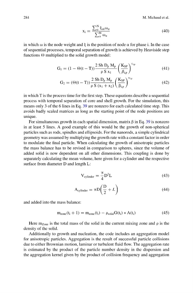
in which ω is the node weight and ξ is the position of node α for phase i. In the case
of sequential processes, temporal separation of growth is achieved by Heaviside step
functions multiplied to the solid growth model:
G 1 = (1 − (t − T))
2 Sh D p M p
ρ S x 1
K SP
β i,p
υ i,p
(41)
G 2 = ((t − T))
2 Sh D p M p
ρ S (x 1 + x 2 )
K SP
β i,p
υ i,p
(42)
in which T is the process time for the first step. These equations describe a sequential
process with temporal separation of core and shell growth. For the simulation, this
means only 3 of the 6 lines in Eq. 39 are nonzero for each calculated time step. This
avoids badly scaled matrices as long as the starting point of the node positions are
unique.
For simultaneous growth in each spatial dimension, matrix β in Eq. 39 is nonzero
in at least 5 lines. A good example of this would be the growth of non-spherical
particles such as rods, spindles and ellipsoids. For the nanorods, a simple cylindrical
geometry was assumed by multiplying the growth rate with a constant factor in order
to modulate the final particle. When calculating the growth of anisotropic particles
the mass balance has to be revised in comparison to spheres, since the volume of
added solid is now dependent on all other dimensions. This coupling is done by
separately calculating the mean volume, here given for a cylinder and the respective
surface from diameter D and length L:
V cylinder =
π
4
D
2 L
(43)
A cylinder = πD
D
2
+ L
(44)
and added into the mass balance:
m zone (t i + 1) = m zone (t i ) − ρ solid G(t i ) ∗ A(t i )
(45)
Here m Zone is the total mass of the solid in the current mixing zone and ρ is the
density of the solid.
Additionally to growth and nucleation, the code includes an aggregation model
for anisotropic particles. Aggregation is the result of successful particle collisions
due to either Brownian motion, laminar or turbulent fluid flow. The aggregation rate
is estimated by the product of the particle number density in the dispersion and
the aggregation kernel given by the product of collision frequency and aggregation
M. Michaud et al.
x i =
N
α ξ αi ω α
N
α ω α
(40)
in which ω is the node weight and ξ is the position of node α for phase i. In the case
of sequential processes, temporal separation of growth is achieved by Heaviside step
functions multiplied to the solid growth model:
G 1 = (1 − (t − T))
2 Sh D p M p
ρ S x 1
K SP
β i,p
υ i,p
(41)
G 2 = ((t − T))
2 Sh D p M p
ρ S (x 1 + x 2 )
K SP
β i,p
υ i,p
(42)
in which T is the process time for the first step. These equations describe a sequential
process with temporal separation of core and shell growth. For the simulation, this
means only 3 of the 6 lines in Eq. 39 are nonzero for each calculated time step. This
avoids badly scaled matrices as long as the starting point of the node positions are
unique.
For simultaneous growth in each spatial dimension, matrix β in Eq. 39 is nonzero
in at least 5 lines. A good example of this would be the growth of non-spherical
particles such as rods, spindles and ellipsoids. For the nanorods, a simple cylindrical
geometry was assumed by multiplying the growth rate with a constant factor in order
to modulate the final particle. When calculating the growth of anisotropic particles
the mass balance has to be revised in comparison to spheres, since the volume of
added solid is now dependent on all other dimensions. This coupling is done by
separately calculating the mean volume, here given for a cylinder and the respective
surface from diameter D and length L:
V cylinder =
π
4
D
2 L
(43)
A cylinder = πD
D
2
+ L
(44)
and added into the mass balance:
m zone (t i + 1) = m zone (t i ) − ρ solid G(t i ) ∗ A(t i )
(45)
Here m Zone is the total mass of the solid in the current mixing zone and ρ is the
density of the solid.
Additionally to growth and nucleation, the code includes an aggregation model
for anisotropic particles. Aggregation is the result of successful particle collisions
due to either Brownian motion, laminar or turbulent fluid flow. The aggregation rate
is estimated by the product of the particle number density in the dispersion and
the aggregation kernel given by the product of collision frequency and aggregation