

8 Flowsheet Simulation of Integrated Precipitation Processes
275
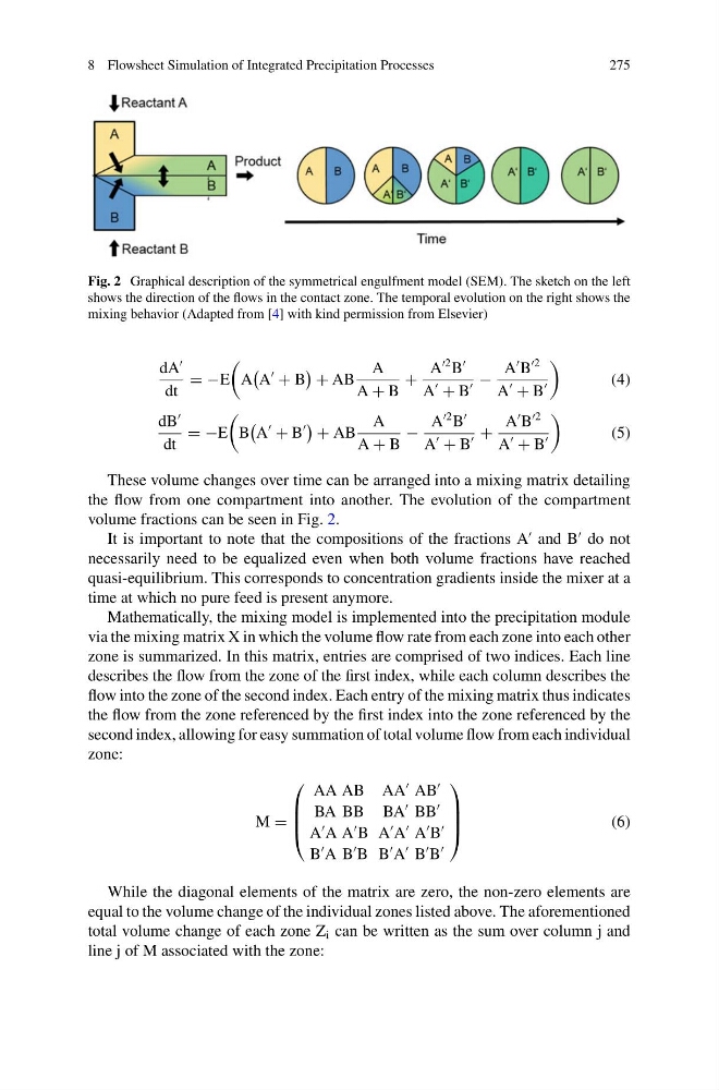
Fig. 2 Graphical description of the symmetrical engulfment model (SEM). The sketch on the left
shows the direction of the flows in the contact zone. The temporal evolution on the right shows the
mixing behavior (Adapted from [4] with kind permission from Elsevier)
dA
dt
= −E
A
A
+ B
+ AB
A
A + B
+
A
2 B
A
+ B
−
A
B
2
A
+ B
(4)
dB
dt
= −E
B
A
+ B
+ AB
A
A + B
−
A
2 B
A
+ B
+
A
B
2
A
+ B
(5)
These volume changes over time can be arranged into a mixing matrix detailing
the flow from one compartment into another. The evolution of the compartment
volume fractions can be seen in Fig. 2.
It is important to note that the compositions of the fractions A
and B
do not
necessarily need to be equalized even when both volume fractions have reached
quasi-equilibrium. This corresponds to concentration gradients inside the mixer at a
time at which no pure feed is present anymore.
Mathematically, the mixing model is implemented into the precipitation module
via the mixing matrix X in which the volume flow rate from each zone into each other
zone is summarized. In this matrix, entries are comprised of two indices. Each line
describes the flow from the zone of the first index, while each column describes the
flow into the zone of the second index. Each entry of the mixing matrix thus indicates
the flow from the zone referenced by the first index into the zone referenced by the
second index, allowing for easy summation of total volume flow from each individual
zone:
M =
⎛
⎜
⎜
⎝
AA AB
BA BB
AA
AB
BA
BB
A
A A
B
B
A B
B
A
A
A
B
B
A
B
B
⎞
⎟
⎟
⎠
(6)
While the diagonal elements of the matrix are zero, the non-zero elements are
equal to the volume change of the individual zones listed above. The aforementioned
total volume change of each zone Z i can be written as the sum over column j and
line j of M associated with the zone:
275
Fig. 2 Graphical description of the symmetrical engulfment model (SEM). The sketch on the left
shows the direction of the flows in the contact zone. The temporal evolution on the right shows the
mixing behavior (Adapted from [4] with kind permission from Elsevier)
dA
dt
= −E
A
A
+ B
+ AB
A
A + B
+
A
2 B
A
+ B
−
A
B
2
A
+ B
(4)
dB
dt
= −E
B
A
+ B
+ AB
A
A + B
−
A
2 B
A
+ B
+
A
B
2
A
+ B
(5)
These volume changes over time can be arranged into a mixing matrix detailing
the flow from one compartment into another. The evolution of the compartment
volume fractions can be seen in Fig. 2.
It is important to note that the compositions of the fractions A
and B
do not
necessarily need to be equalized even when both volume fractions have reached
quasi-equilibrium. This corresponds to concentration gradients inside the mixer at a
time at which no pure feed is present anymore.
Mathematically, the mixing model is implemented into the precipitation module
via the mixing matrix X in which the volume flow rate from each zone into each other
zone is summarized. In this matrix, entries are comprised of two indices. Each line
describes the flow from the zone of the first index, while each column describes the
flow into the zone of the second index. Each entry of the mixing matrix thus indicates
the flow from the zone referenced by the first index into the zone referenced by the
second index, allowing for easy summation of total volume flow from each individual
zone:
M =
⎛
⎜
⎜
⎝
AA AB
BA BB
AA
AB
BA
BB
A
A A
B
B
A B
B
A
A
A
B
B
A
B
B
⎞
⎟
⎟
⎠
(6)
While the diagonal elements of the matrix are zero, the non-zero elements are
equal to the volume change of the individual zones listed above. The aforementioned
total volume change of each zone Z i can be written as the sum over column j and
line j of M associated with the zone: