

246
M. Gleiss and H. Nirschl
F(D) =
D
0
E(D)d D.
(4)
For the mean residence time D = 1, the residence time spectrum reaches its
maximum and the residence time distribution reaches the mean value.
The right side in Fig. 4 illustrates the comparison of the real residence time
behavior with an ideal plug flow reactor (PFR) and a continuous stirred tank reactor
(CSTR). PFR modeling assumes, that the flow is uniform and there is no exchange
of forces along the cross-section. This results in a sudden change of the residence
time behavior after reaching the mean residence time. CSTR modeling supposes
no gradients in the apparatus and the change occurring immediately at the output.
This leads to a broad sum distribution with high axial dispersion. Real processes
generally differ significantly from the performance of a PFR and CSTR, see Figs. 1
and 4, because the axial dispersion depends on the flow conditions. Dead zones and
back-mixing are present inside centrifuges. Consequently, the real residence time
behavior of a process differs considerable from ideal behavior.
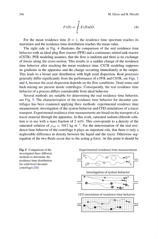
Several methods are suitable for determining the real residence time behavior,
see Fig. 5. The characterization of the residence time behavior for decanter centrifuges has been examined applying three methods: experimental residence time
measurement, investigation of the system behavior and CFD simulations of a tracer
transport. Experimental residence time measurements are based on the transport of a
tracer material through the apparatus. In this work, saturated sodium-chloride solution is in use with a mass fraction of 2 wt%. This corresponds to a density of the
saturated solution of ρ sol = 1012 kg m
−3 . For the determination of the real residence time behavior of the centrifuge it plays an important role, that there is only a
neglectable difference in density between the liquid and the tracer. Otherwise segregation of the two fluids occur due to the acting g-force. At this point it should be
Fig. 5 Comparison of the
investigated three different
methods to determine the
residence time distribution
for solid-bowl decanter
centrifuges [20]
M. Gleiss and H. Nirschl
F(D) =
D
0
E(D)d D.
(4)
For the mean residence time D = 1, the residence time spectrum reaches its
maximum and the residence time distribution reaches the mean value.
The right side in Fig. 4 illustrates the comparison of the real residence time
behavior with an ideal plug flow reactor (PFR) and a continuous stirred tank reactor
(CSTR). PFR modeling assumes, that the flow is uniform and there is no exchange
of forces along the cross-section. This results in a sudden change of the residence
time behavior after reaching the mean residence time. CSTR modeling supposes
no gradients in the apparatus and the change occurring immediately at the output.
This leads to a broad sum distribution with high axial dispersion. Real processes
generally differ significantly from the performance of a PFR and CSTR, see Figs. 1
and 4, because the axial dispersion depends on the flow conditions. Dead zones and
back-mixing are present inside centrifuges. Consequently, the real residence time
behavior of a process differs considerable from ideal behavior.
Several methods are suitable for determining the real residence time behavior,
see Fig. 5. The characterization of the residence time behavior for decanter centrifuges has been examined applying three methods: experimental residence time
measurement, investigation of the system behavior and CFD simulations of a tracer
transport. Experimental residence time measurements are based on the transport of a
tracer material through the apparatus. In this work, saturated sodium-chloride solution is in use with a mass fraction of 2 wt%. This corresponds to a density of the
saturated solution of ρ sol = 1012 kg m
−3 . For the determination of the real residence time behavior of the centrifuge it plays an important role, that there is only a
neglectable difference in density between the liquid and the tracer. Otherwise segregation of the two fluids occur due to the acting g-force. At this point it should be
Fig. 5 Comparison of the
investigated three different
methods to determine the
residence time distribution
for solid-bowl decanter
centrifuges [20]