

4 Dynamic Simulation of Technical Precipitation Processes
123
A
B
B
A
M
B
A
M
M
z
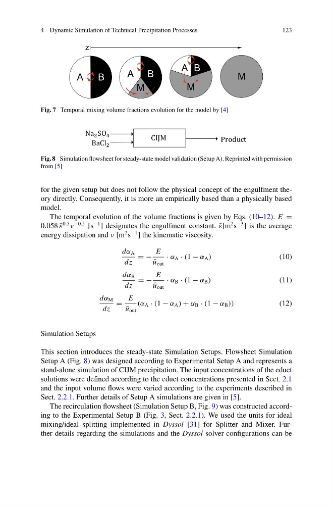
Fig. 7 Temporal mixing volume fractions evolution for the model by [4]
Fig. 8 Simulation flowsheet for steady-state model validation (Setup A). Reprinted with permission
from [5]
for the given setup but does not follow the physical concept of the engulfment theory directly. Consequently, it is more an empirically based than a physically based
model.
The temporal evolution of the volume fractions is given by Eqs. (10–12). E =
0.058 ¯
ε
0.5
ν
−0.5
[s
−1
] designates the engulfment constant. ¯
ε[m
2 s
−3
] is the average
energy dissipation and ν [m
2 s
−1
] the kinematic viscosity.
dα A
dz
= −
E
¯
u out
· α A · (1 − α A )
(10)
dα B
dz
= −
E
¯
u out
· α B · (1 − α B )
(11)
dα M
dz
=
E
¯
u out
(α A · (1 − α A ) + α B · (1 − α B ))
(12)
Simulation Setups
This section introduces the steady-state Simulation Setups. Flowsheet Simulation
Setup A (Fig. 8) was designed according to Experimental Setup A and represents a
stand-alone simulation of CIJM precipitation. The input concentrations of the educt
solutions were defined according to the educt concentrations presented in Sect. 2.1
and the input volume flows were varied according to the experiments described in
Sect. 2.2.1. Further details of Setup A simulations are given in [5].
The recirculation flowsheet (Simulation Setup B, Fig. 9) was constructed according to the Experimental Setup B (Fig. 3, Sect. 2.2.1). We used the units for ideal
mixing/ideal splitting implemented in Dyssol [31] for Splitter and Mixer. Further details regarding the simulations and the Dyssol solver configurations can be
123
A
B
B
A
M
B
A
M
M
z
Fig. 7 Temporal mixing volume fractions evolution for the model by [4]
Fig. 8 Simulation flowsheet for steady-state model validation (Setup A). Reprinted with permission
from [5]
for the given setup but does not follow the physical concept of the engulfment theory directly. Consequently, it is more an empirically based than a physically based
model.
The temporal evolution of the volume fractions is given by Eqs. (10–12). E =
0.058 ¯
ε
0.5
ν
−0.5
[s
−1
] designates the engulfment constant. ¯
ε[m
2 s
−3
] is the average
energy dissipation and ν [m
2 s
−1
] the kinematic viscosity.
dα A
dz
= −
E
¯
u out
· α A · (1 − α A )
(10)
dα B
dz
= −
E
¯
u out
· α B · (1 − α B )
(11)
dα M
dz
=
E
¯
u out
(α A · (1 − α A ) + α B · (1 − α B ))
(12)
Simulation Setups
This section introduces the steady-state Simulation Setups. Flowsheet Simulation
Setup A (Fig. 8) was designed according to Experimental Setup A and represents a
stand-alone simulation of CIJM precipitation. The input concentrations of the educt
solutions were defined according to the educt concentrations presented in Sect. 2.1
and the input volume flows were varied according to the experiments described in
Sect. 2.2.1. Further details of Setup A simulations are given in [5].
The recirculation flowsheet (Simulation Setup B, Fig. 9) was constructed according to the Experimental Setup B (Fig. 3, Sect. 2.2.1). We used the units for ideal
mixing/ideal splitting implemented in Dyssol [31] for Splitter and Mixer. Further details regarding the simulations and the Dyssol solver configurations can be