

122
H. Rehage and M. Kind
¯
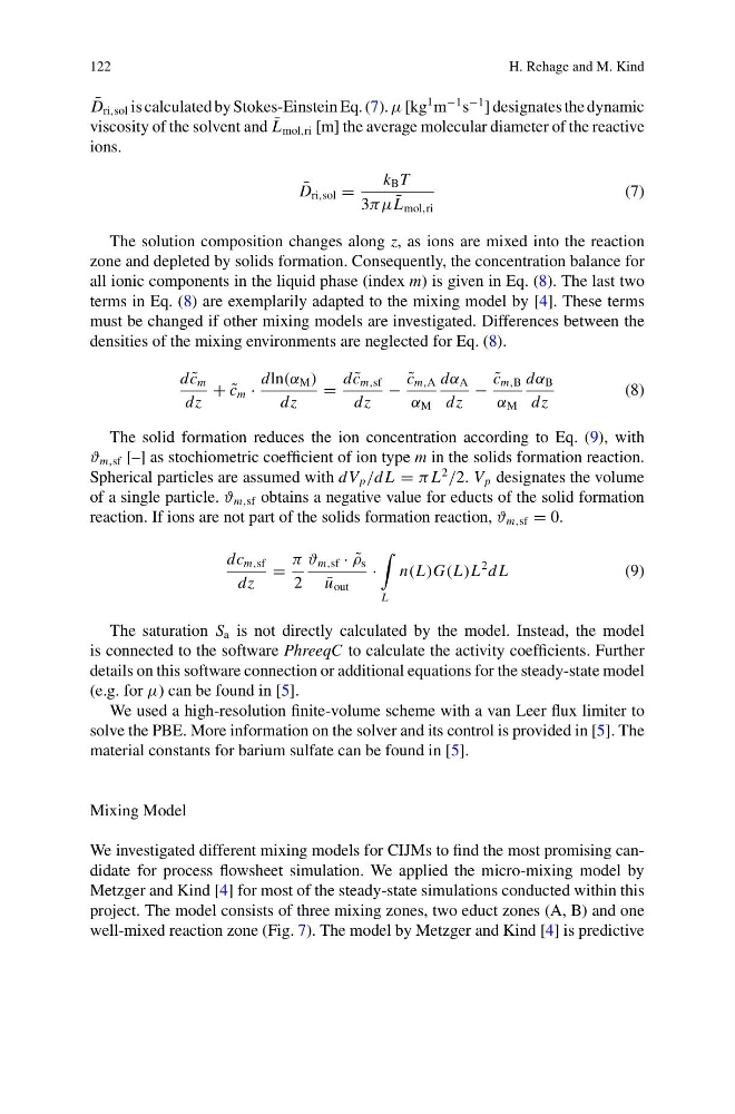
D ri,sol is calculated by Stokes-Einstein Eq. (7). μ [kg
1 m
−1 s
−1
] designates the dynamic
viscosity of the solvent and ¯
L mol,ri [m] the average molecular diameter of the reactive
ions.
¯
D ri,sol =
k B T
3πμ ¯
L mol,ri
(7)
The solution composition changes along z, as ions are mixed into the reaction
zone and depleted by solids formation. Consequently, the concentration balance for
all ionic components in the liquid phase (index m) is given in Eq. (8). The last two
terms in Eq. (8) are exemplarily adapted to the mixing model by [4]. These terms
must be changed if other mixing models are investigated. Differences between the
densities of the mixing environments are neglected for Eq. (8).
d ˜
c m
dz
+ ˜
c m ·
dln(α M )
dz
=
d ˜
c m,sf
dz
−
˜
c m,A
α M
dα A
dz
−
˜
c m,B
α M
dα B
dz
(8)
The solid formation reduces the ion concentration according to Eq. (9), with
ϑ m,sf [–] as stochiometric coefficient of ion type m in the solids formation reaction.
Spherical particles are assumed with dV p /d L = π L
2
/2. V p designates the volume
of a single particle. ϑ m,sf obtains a negative value for educts of the solid formation
reaction. If ions are not part of the solids formation reaction, ϑ m,sf = 0.
dc m,sf
dz
=
π
2
ϑ m,sf · ˜
ρ s
¯
u out
·
L
n(L)G(L)L
2 d L
(9)
The saturation S a is not directly calculated by the model. Instead, the model
is connected to the software PhreeqC to calculate the activity coefficients. Further
details on this software connection or additional equations for the steady-state model
(e.g. for μ) can be found in [5].
We used a high-resolution finite-volume scheme with a van Leer flux limiter to
solve the PBE. More information on the solver and its control is provided in [5]. The
material constants for barium sulfate can be found in [5].
Mixing Model
We investigated different mixing models for CIJMs to find the most promising candidate for process flowsheet simulation. We applied the micro-mixing model by
Metzger and Kind [4] for most of the steady-state simulations conducted within this
project. The model consists of three mixing zones, two educt zones (A, B) and one
well-mixed reaction zone (Fig. 7). The model by Metzger and Kind [4] is predictive
H. Rehage and M. Kind
¯
D ri,sol is calculated by Stokes-Einstein Eq. (7). μ [kg
1 m
−1 s
−1
] designates the dynamic
viscosity of the solvent and ¯
L mol,ri [m] the average molecular diameter of the reactive
ions.
¯
D ri,sol =
k B T
3πμ ¯
L mol,ri
(7)
The solution composition changes along z, as ions are mixed into the reaction
zone and depleted by solids formation. Consequently, the concentration balance for
all ionic components in the liquid phase (index m) is given in Eq. (8). The last two
terms in Eq. (8) are exemplarily adapted to the mixing model by [4]. These terms
must be changed if other mixing models are investigated. Differences between the
densities of the mixing environments are neglected for Eq. (8).
d ˜
c m
dz
+ ˜
c m ·
dln(α M )
dz
=
d ˜
c m,sf
dz
−
˜
c m,A
α M
dα A
dz
−
˜
c m,B
α M
dα B
dz
(8)
The solid formation reduces the ion concentration according to Eq. (9), with
ϑ m,sf [–] as stochiometric coefficient of ion type m in the solids formation reaction.
Spherical particles are assumed with dV p /d L = π L
2
/2. V p designates the volume
of a single particle. ϑ m,sf obtains a negative value for educts of the solid formation
reaction. If ions are not part of the solids formation reaction, ϑ m,sf = 0.
dc m,sf
dz
=
π
2
ϑ m,sf · ˜
ρ s
¯
u out
·
L
n(L)G(L)L
2 d L
(9)
The saturation S a is not directly calculated by the model. Instead, the model
is connected to the software PhreeqC to calculate the activity coefficients. Further
details on this software connection or additional equations for the steady-state model
(e.g. for μ) can be found in [5].
We used a high-resolution finite-volume scheme with a van Leer flux limiter to
solve the PBE. More information on the solver and its control is provided in [5]. The
material constants for barium sulfate can be found in [5].
Mixing Model
We investigated different mixing models for CIJMs to find the most promising candidate for process flowsheet simulation. We applied the micro-mixing model by
Metzger and Kind [4] for most of the steady-state simulations conducted within this
project. The model consists of three mixing zones, two educt zones (A, B) and one
well-mixed reaction zone (Fig. 7). The model by Metzger and Kind [4] is predictive