

554
15 Random Vibrations
The treatment for finite element random analysis of plates is similar to that of
multiple degrees of freedom system.
Let us express the displacements in terms of normal coordinates
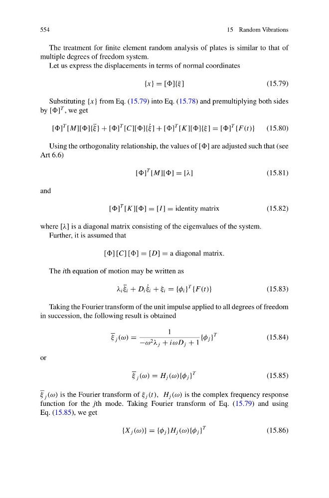
{x} = []{ξ ]
(15.79)
Substituting {x} from Eq. (15.79) into Eq. (15.78) and premultiplying both sides
by []
T , we get
[]
T
[M][]{ ¨
ξ } + []
T
[C][]{ ˙
ξ ] + []
T
[K ][]{ξ ] = []
T
{F(t)}
(15.80)
Using the orthogonality relationship, the values of [] are adjusted such that (see
Art 6.6)
[]
T
[M][] = [λ]
(15.81)
and
[]
T
[K ][] = [I ] = identity matrix
(15.82)
where [λ] is a diagonal matrix consisting of the eigenvalues of the system.
Further, it is assumed that
[] [C] [] = [D] = a diagonal matrix.
The ith equation of motion may be written as
λ i ¨
ξ i + D i ˙
ξ i + ξ i = {φ i }
T
{F(t)}
(15.83)
Taking the Fourier transform of the unit impulse applied to all degrees of freedom
in succession, the following result is obtained
ξ j (ω) =
1
−ω 2 λ j + iωD j + 1
{φ j }
T
(15.84)
or
ξ j (ω) = H j (ω){φ j }
T
(15.85)
ξ j (ω) is the Fourier transform of ξ j (t), H j (ω) is the complex frequency response
function for the jth mode. Taking Fourier transform of Eq. (15.79) and using
Eq. (15.85), we get
{X j (ω)} = {φ j }H j (ω){φ j }
T
(15.86)
15 Random Vibrations
The treatment for finite element random analysis of plates is similar to that of
multiple degrees of freedom system.
Let us express the displacements in terms of normal coordinates
{x} = []{ξ ]
(15.79)
Substituting {x} from Eq. (15.79) into Eq. (15.78) and premultiplying both sides
by []
T , we get
[]
T
[M][]{ ¨
ξ } + []
T
[C][]{ ˙
ξ ] + []
T
[K ][]{ξ ] = []
T
{F(t)}
(15.80)
Using the orthogonality relationship, the values of [] are adjusted such that (see
Art 6.6)
[]
T
[M][] = [λ]
(15.81)
and
[]
T
[K ][] = [I ] = identity matrix
(15.82)
where [λ] is a diagonal matrix consisting of the eigenvalues of the system.
Further, it is assumed that
[] [C] [] = [D] = a diagonal matrix.
The ith equation of motion may be written as
λ i ¨
ξ i + D i ˙
ξ i + ξ i = {φ i }
T
{F(t)}
(15.83)
Taking the Fourier transform of the unit impulse applied to all degrees of freedom
in succession, the following result is obtained
ξ j (ω) =
1
−ω 2 λ j + iωD j + 1
{φ j }
T
(15.84)
or
ξ j (ω) = H j (ω){φ j }
T
(15.85)
ξ j (ω) is the Fourier transform of ξ j (t), H j (ω) is the complex frequency response
function for the jth mode. Taking Fourier transform of Eq. (15.79) and using
Eq. (15.85), we get
{X j (ω)} = {φ j }H j (ω){φ j }
T
(15.86)