

552
15 Random Vibrations
S ξ 2 ξ 1 = H
∗
1 (ω)H 2 (ω)S 0 , S ξ 2 ξ 1 = H 2 (ω)
2 S 0
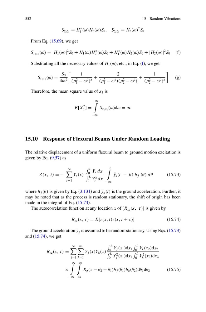
From Eq. (15.69), we get
S x 1 x 1 (ω) = |H 1 (ω)|
2 S 0 + H 1 (ω)H
∗
2 (ω)S 0 + H
∗
1 (ω)H 2 (ω)S 0 + |H 2 (ω)|
2 S 0 (f)
Substituting all the necessary values of H 1 (ω), etc., in Eq. (f), we get
S x 1 x 1 (ω) =
S 0
4m 2
1
( p
2
1 − ω 2 ) 2 +
2
( p
2
1 − ω 2 )( p
2
2 − ω 2 )
+
1
( p
2
2 − ω 2 ) 2
(g)
Therefore, the mean square value of x 1 is
E[X
2
1 ] =
∞
−∞
S x 1 x 1 (ω)dω = ∞
15.10 Response of Flexural Beams Under Random Loading
The relative displacement of a uniform flexural beam to ground motion excitation is
given by Eq. (9.57) as
Z (x, t) = −
∞
r =1
Y r (x)
L
0 Y r dx
L
0 Y 2
r dx
t
− ∞
¨
y s (t − θ) h j (θ ) dθ
(15.73)
where h j (θ ) is given by Eq. (3.131) and ¨
y g (t) is the ground acceleration. Further, it
may be noted that as the process is random stationary, the shift of origin has been
made in the integral of Eq. (15.73).
The autocorrelation function at any location x of [R zz (x, τ)] is given by
R zz (x, τ ) = E[z(x, t)z(x, t + τ )]
(15.74)
The ground acceleration ¨
y g is assumed to be random stationary. Using Eqs. (15.73)
and (15.74), we get
R zz (x, τ ) =
∞
j=1
∞
k=1
Y j (x)Y k (x)
L
0 Y j (x 1 )dx 1
L
0 Y k (x 2 )dx 2
L
0 Y
2
j (x 1 )dx 1
L
0 Y
2
k (x 2 )dx 2
×
∞
−∞
∞
−∞
R g (τ − θ 2 + θ 1 )h j (θ 1 )h k (θ 2 )dθ 1 dθ 2
(15.75)
15 Random Vibrations
S ξ 2 ξ 1 = H
∗
1 (ω)H 2 (ω)S 0 , S ξ 2 ξ 1 = H 2 (ω)
2 S 0
From Eq. (15.69), we get
S x 1 x 1 (ω) = |H 1 (ω)|
2 S 0 + H 1 (ω)H
∗
2 (ω)S 0 + H
∗
1 (ω)H 2 (ω)S 0 + |H 2 (ω)|
2 S 0 (f)
Substituting all the necessary values of H 1 (ω), etc., in Eq. (f), we get
S x 1 x 1 (ω) =
S 0
4m 2
1
( p
2
1 − ω 2 ) 2 +
2
( p
2
1 − ω 2 )( p
2
2 − ω 2 )
+
1
( p
2
2 − ω 2 ) 2
(g)
Therefore, the mean square value of x 1 is
E[X
2
1 ] =
∞
−∞
S x 1 x 1 (ω)dω = ∞
15.10 Response of Flexural Beams Under Random Loading
The relative displacement of a uniform flexural beam to ground motion excitation is
given by Eq. (9.57) as
Z (x, t) = −
∞
r =1
Y r (x)
L
0 Y r dx
L
0 Y 2
r dx
t
− ∞
¨
y s (t − θ) h j (θ ) dθ
(15.73)
where h j (θ ) is given by Eq. (3.131) and ¨
y g (t) is the ground acceleration. Further, it
may be noted that as the process is random stationary, the shift of origin has been
made in the integral of Eq. (15.73).
The autocorrelation function at any location x of [R zz (x, τ)] is given by
R zz (x, τ ) = E[z(x, t)z(x, t + τ )]
(15.74)
The ground acceleration ¨
y g is assumed to be random stationary. Using Eqs. (15.73)
and (15.74), we get
R zz (x, τ ) =
∞
j=1
∞
k=1
Y j (x)Y k (x)
L
0 Y j (x 1 )dx 1
L
0 Y k (x 2 )dx 2
L
0 Y
2
j (x 1 )dx 1
L
0 Y
2
k (x 2 )dx 2
×
∞
−∞
∞
−∞
R g (τ − θ 2 + θ 1 )h j (θ 1 )h k (θ 2 )dθ 1 dθ 2
(15.75)