

550
15 Random Vibrations
The spectral densities in terms of the original coordinate system can be related to
modal spectral densities as follows:
S x i x j ( f ) =
n
r =1
n
s=1
φ
(r )
i φ
(s)
i S ξ r ξ s ( f )
(15.69)
Sometimes it is convenient to note the following relationship
S ξ r ξ s ( f ) = S
∗
ξ r ξ s
( f ) for r = s
(15.70)
Using the relation given by Eq. (15.70), Eq. (15.69) is rewritten for direct spectral
densities as
S x i x j ( f ) =
n
r =1
(φ
(r )
i )
2 S ξ i ξ j ( f ) + 2
n
r =1
n
s=1
φ
(r )
i φ
(s)
i Re {S ξ r ξ s ( f )}
(15.71)
where Re{} denotes the real part of the function. Further, for most practical problems,
second term on the right-hand side of Eq. (15.71) may be neglected. Substituting
S ξ i ξ j ( f ) from Eq. (15.68) into Eq. (15.69) will give the element S x i x j ( f ) of the
spectral density matrix. Computing all such elements, the spectral density matrix
can be written as
[S xx ( f )] = [] [H ( f )] []
T
[S F F ( f )] [] [H ( f )] []
T
(15.72)
Once the spectral densities are obtained, the mean square value of the response
can be derived by following the same procedure as mentioned earlier.
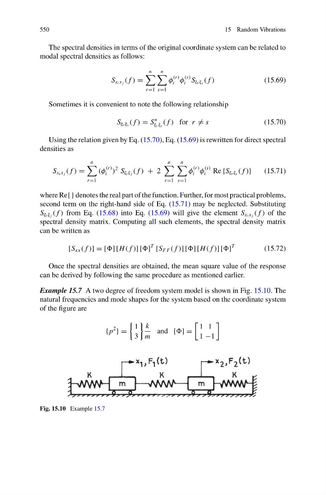
Example 15.7 A two degree of freedom system model is shown in Fig. 15.10. The
natural frequencies and mode shapes for the system based on the coordinate system
of the figure are
{ p
2
} =
1
3
k
m
and [] =
1 1
1 −1
Fig. 15.10 Example 15.7
15 Random Vibrations
The spectral densities in terms of the original coordinate system can be related to
modal spectral densities as follows:
S x i x j ( f ) =
n
r =1
n
s=1
φ
(r )
i φ
(s)
i S ξ r ξ s ( f )
(15.69)
Sometimes it is convenient to note the following relationship
S ξ r ξ s ( f ) = S
∗
ξ r ξ s
( f ) for r = s
(15.70)
Using the relation given by Eq. (15.70), Eq. (15.69) is rewritten for direct spectral
densities as
S x i x j ( f ) =
n
r =1
(φ
(r )
i )
2 S ξ i ξ j ( f ) + 2
n
r =1
n
s=1
φ
(r )
i φ
(s)
i Re {S ξ r ξ s ( f )}
(15.71)
where Re{} denotes the real part of the function. Further, for most practical problems,
second term on the right-hand side of Eq. (15.71) may be neglected. Substituting
S ξ i ξ j ( f ) from Eq. (15.68) into Eq. (15.69) will give the element S x i x j ( f ) of the
spectral density matrix. Computing all such elements, the spectral density matrix
can be written as
[S xx ( f )] = [] [H ( f )] []
T
[S F F ( f )] [] [H ( f )] []
T
(15.72)
Once the spectral densities are obtained, the mean square value of the response
can be derived by following the same procedure as mentioned earlier.
Example 15.7 A two degree of freedom system model is shown in Fig. 15.10. The
natural frequencies and mode shapes for the system based on the coordinate system
of the figure are
{ p
2
} =
1
3
k
m
and [] =
1 1
1 −1
Fig. 15.10 Example 15.7