

15.9 Random Response of MDF Systems
549
15.9.2 Normal Mode Method
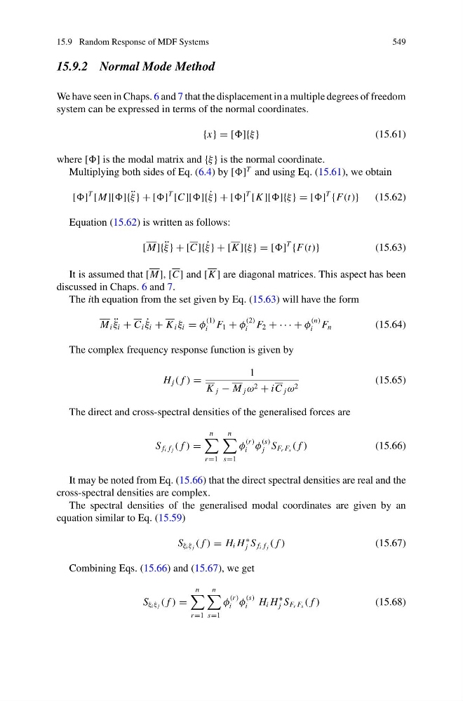
We have seen in Chaps. 6 and 7 that the displacement in a multiple degrees of freedom
system can be expressed in terms of the normal coordinates.
{x} = []{ξ }
(15.61)
where [] is the modal matrix and {ξ } is the normal coordinate.
Multiplying both sides of Eq. (6.4) by []
T and using Eq. (15.61), we obtain
[]
T
[M][]{ ¨
ξ } + []
T
[C][]{ ˙
ξ } + []
T
[K ][]{ξ } = []
T
{F(t)}
(15.62)
Equation (15.62) is written as follows:
[M]{ ¨
ξ } + [C]{ ˙
ξ } + [K ]{ξ } = []
T
{F(t)}
(15.63)
It is assumed that [M], [C] and [K ] are diagonal matrices. This aspect has been
discussed in Chaps. 6 and 7.
The ith equation from the set given by Eq. (15.63) will have the form
M i ¨
ξ i + C i ˙
ξ i + K i ξ i = φ
(1)
i F 1 + φ
(2)
i F 2 + · · · + φ
(n)
i F n
(15.64)
The complex frequency response function is given by
H j ( f ) =
1
K j − M j ω 2 + iC j ω 2
(15.65)
The direct and cross-spectral densities of the generalised forces are
S f i f j ( f ) =
n
r =1
n
s=1
φ
(r )
i φ
(s)
j S F r F s ( f )
(15.66)
It may be noted from Eq. (15.66) that the direct spectral densities are real and the
cross-spectral densities are complex.
The spectral densities of the generalised modal coordinates are given by an
equation similar to Eq. (15.59)
S ξ i ξ j ( f ) = H i H
∗
j S f i f j ( f )
(15.67)
Combining Eqs. (15.66) and (15.67), we get
S ξ i ξ j ( f ) =
n
r =1
n
s=1
φ
(r )
i φ
(s)
i
H i H
∗
j S F r F s ( f )
(15.68)
549
15.9.2 Normal Mode Method
We have seen in Chaps. 6 and 7 that the displacement in a multiple degrees of freedom
system can be expressed in terms of the normal coordinates.
{x} = []{ξ }
(15.61)
where [] is the modal matrix and {ξ } is the normal coordinate.
Multiplying both sides of Eq. (6.4) by []
T and using Eq. (15.61), we obtain
[]
T
[M][]{ ¨
ξ } + []
T
[C][]{ ˙
ξ } + []
T
[K ][]{ξ } = []
T
{F(t)}
(15.62)
Equation (15.62) is written as follows:
[M]{ ¨
ξ } + [C]{ ˙
ξ } + [K ]{ξ } = []
T
{F(t)}
(15.63)
It is assumed that [M], [C] and [K ] are diagonal matrices. This aspect has been
discussed in Chaps. 6 and 7.
The ith equation from the set given by Eq. (15.63) will have the form
M i ¨
ξ i + C i ˙
ξ i + K i ξ i = φ
(1)
i F 1 + φ
(2)
i F 2 + · · · + φ
(n)
i F n
(15.64)
The complex frequency response function is given by
H j ( f ) =
1
K j − M j ω 2 + iC j ω 2
(15.65)
The direct and cross-spectral densities of the generalised forces are
S f i f j ( f ) =
n
r =1
n
s=1
φ
(r )
i φ
(s)
j S F r F s ( f )
(15.66)
It may be noted from Eq. (15.66) that the direct spectral densities are real and the
cross-spectral densities are complex.
The spectral densities of the generalised modal coordinates are given by an
equation similar to Eq. (15.59)
S ξ i ξ j ( f ) = H i H
∗
j S f i f j ( f )
(15.67)
Combining Eqs. (15.66) and (15.67), we get
S ξ i ξ j ( f ) =
n
r =1
n
s=1
φ
(r )
i φ
(s)
i
H i H
∗
j S F r F s ( f )
(15.68)