

15.7 Relationship Between Autocorrelation Function and Power Spectral Density
541
φ(τ ) = lim
T →∞
1
T
∞
−∞
F( f )
⎡
⎢
⎣
T /2
−T /2
F(t)e
i2π f t dt
⎤
⎥
⎦e
i2π f τ d f
(15.35)
Combining Eqs. (15.28) and (15.35), we get
φ(τ ) = lim
T →∞
∞
−∞
1
T
F( f )F ∗ ( f ) e
i2π f τ dt
or
φ(τ ) = lim
T →∞
∞
−∞
1
T
|F( f )|
2 e
i2π f τ d f
(15.36)
Combining Eqs. (15.31) and (15.36), we get
φ(τ ) =
∞
−∞
S( f ) e
i2π f τ d f
(15.37)
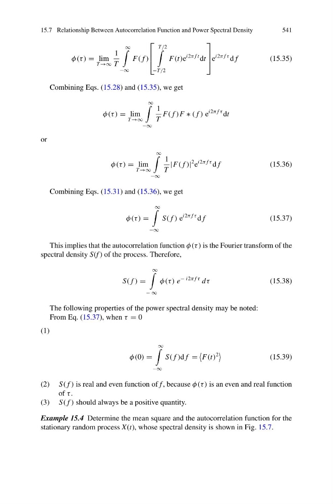
This implies that the autocorrelation function φ(τ ) is the Fourier transform of the
spectral density S(f ) of the process. Therefore,
S( f ) =
∞
− ∞
φ(τ ) e
− i2π f τ dτ
(15.38)
The following properties of the power spectral density may be noted:
From Eq. (15.37), when τ = 0
(1)
φ(0) =
∞
−∞
S( f )d f =
F(t)
2
(15.39)
(2) S( f ) is real and even function of f , because φ(τ ) is an even and real function
of τ .
(3) S( f ) should always be a positive quantity.
Example 15.4 Determine the mean square and the autocorrelation function for the
stationary random process X(t), whose spectral density is shown in Fig. 15.7.
541
φ(τ ) = lim
T →∞
1
T
∞
−∞
F( f )
⎡
⎢
⎣
T /2
−T /2
F(t)e
i2π f t dt
⎤
⎥
⎦e
i2π f τ d f
(15.35)
Combining Eqs. (15.28) and (15.35), we get
φ(τ ) = lim
T →∞
∞
−∞
1
T
F( f )F ∗ ( f ) e
i2π f τ dt
or
φ(τ ) = lim
T →∞
∞
−∞
1
T
|F( f )|
2 e
i2π f τ d f
(15.36)
Combining Eqs. (15.31) and (15.36), we get
φ(τ ) =
∞
−∞
S( f ) e
i2π f τ d f
(15.37)
This implies that the autocorrelation function φ(τ ) is the Fourier transform of the
spectral density S(f ) of the process. Therefore,
S( f ) =
∞
− ∞
φ(τ ) e
− i2π f τ dτ
(15.38)
The following properties of the power spectral density may be noted:
From Eq. (15.37), when τ = 0
(1)
φ(0) =
∞
−∞
S( f )d f =
F(t)
2
(15.39)
(2) S( f ) is real and even function of f , because φ(τ ) is an even and real function
of τ .
(3) S( f ) should always be a positive quantity.
Example 15.4 Determine the mean square and the autocorrelation function for the
stationary random process X(t), whose spectral density is shown in Fig. 15.7.