

532
15 Random Vibrations
p(x 1 ) =
∞
− ∞
p(x 1 , x 2 )dx 2
(15.8)
or likewise
p(x 2 ) =
∞
−∞
p(x 1 , x 2 )dx 1
(15.9)
The derivation of Eqs. (15.8) and (15.9) is left as an exercise to the reader.
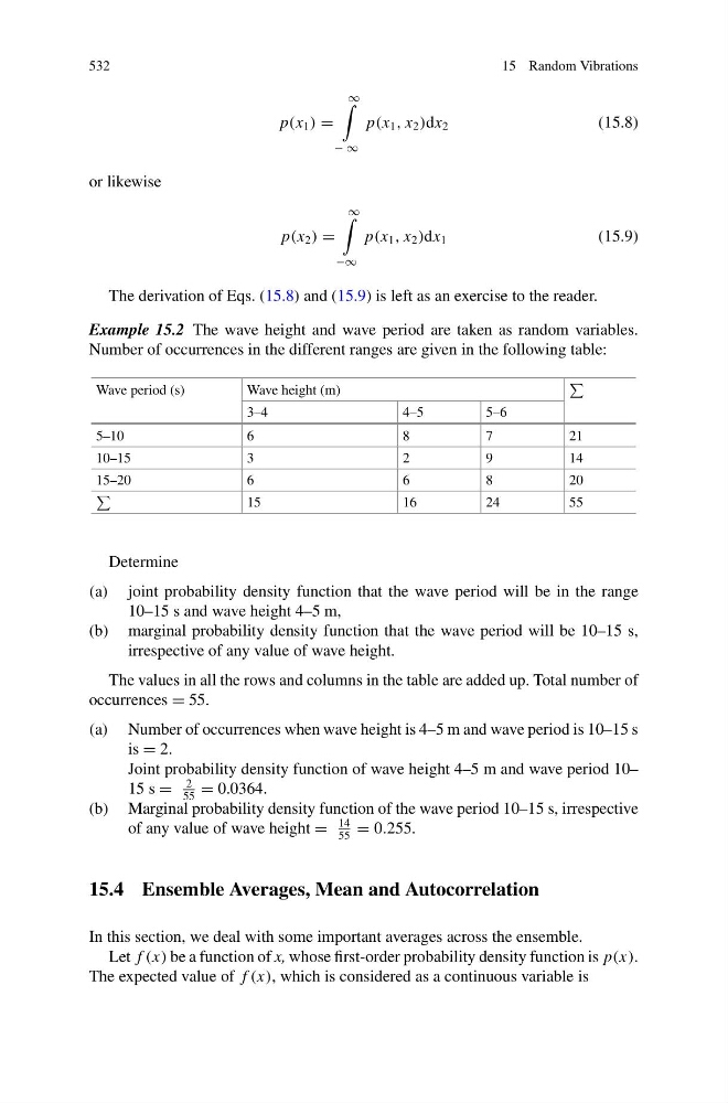
Example 15.2 The wave height and wave period are taken as random variables.
Number of occurrences in the different ranges are given in the following table:
Wave period (s)
Wave height (m)
3–4
4–5
5–6
5–10
6
8
7
21
10–15
3
2
9
14
15–20
6
6
8
20
15
16
24
55
Determine
(a) joint probability density function that the wave period will be in the range
10–15 s and wave height 4–5 m,
(b) marginal probability density function that the wave period will be 10–15 s,
irrespective of any value of wave height.
The values in all the rows and columns in the table are added up. Total number of
occurrences = 55.
(a) Number of occurrences when wave height is 4–5 m and wave period is 10–15 s
is = 2.
Joint probability density function of wave height 4–5 m and wave period 10–
15 s =
2
55
= 0.0364.
(b) Marginal probability density function of the wave period 10–15 s, irrespective
of any value of wave height =
14
55
= 0.255.
15.4 Ensemble Averages, Mean and Autocorrelation
In this section, we deal with some important averages across the ensemble.
Let f (x) be a function of x, whose first-order probability density function is p(x).
The expected value of f (x), which is considered as a continuous variable is
15 Random Vibrations
p(x 1 ) =
∞
− ∞
p(x 1 , x 2 )dx 2
(15.8)
or likewise
p(x 2 ) =
∞
−∞
p(x 1 , x 2 )dx 1
(15.9)
The derivation of Eqs. (15.8) and (15.9) is left as an exercise to the reader.
Example 15.2 The wave height and wave period are taken as random variables.
Number of occurrences in the different ranges are given in the following table:
Wave period (s)
Wave height (m)
3–4
4–5
5–6
5–10
6
8
7
21
10–15
3
2
9
14
15–20
6
6
8
20
15
16
24
55
Determine
(a) joint probability density function that the wave period will be in the range
10–15 s and wave height 4–5 m,
(b) marginal probability density function that the wave period will be 10–15 s,
irrespective of any value of wave height.
The values in all the rows and columns in the table are added up. Total number of
occurrences = 55.
(a) Number of occurrences when wave height is 4–5 m and wave period is 10–15 s
is = 2.
Joint probability density function of wave height 4–5 m and wave period 10–
15 s =
2
55
= 0.0364.
(b) Marginal probability density function of the wave period 10–15 s, irrespective
of any value of wave height =
14
55
= 0.255.
15.4 Ensemble Averages, Mean and Autocorrelation
In this section, we deal with some important averages across the ensemble.
Let f (x) be a function of x, whose first-order probability density function is p(x).
The expected value of f (x), which is considered as a continuous variable is