

530
15 Random Vibrations
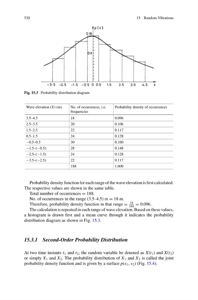
Fig. 15.3 Probability distribution diagram
Wave elevation (X) (m)
No. of occurrences, i.e.
frequencies
Probability density of occurrences
3.5–4.5
18
0.096
2.5–3.5
20
0.106
1.5–2.5
22
0.117
0.5–1.5
24
0.128
−0.5–0.5
30
0.160
−1.5–(−0.5)
28
0.148
−2.5–(−1.5)
24
0.128
−3.5–(−2.5)
22
0.117
188
1.000
Probability density function for each range of the wave elevation is first calculated.
The respective values are shown in the same table.
Total number of occurrences = 188.
No. of occurrences in the range (3.5–4.5) m = 18 m.
Therefore, probability density function in that range =
18
188
= 0.096.
The calculation is repeated in each range of wave elevation. Based on these values,
a histogram is drawn first and a mean curve through it indicates the probability
distribution diagram as shown in Fig. 15.3.
15.3.1 Second-Order Probability Distribution
At two time instants t 1 and t 2 , the random variable be denoted as X(t 1 ) and X(t 2 )
or simply X 1 and X 2 . The probability distribution of X 1 and X 2 is called the joint
probability density function and is given by a surface p(x 1 , x 2 ) (Fig. 15.4).
15 Random Vibrations
Fig. 15.3 Probability distribution diagram
Wave elevation (X) (m)
No. of occurrences, i.e.
frequencies
Probability density of occurrences
3.5–4.5
18
0.096
2.5–3.5
20
0.106
1.5–2.5
22
0.117
0.5–1.5
24
0.128
−0.5–0.5
30
0.160
−1.5–(−0.5)
28
0.148
−2.5–(−1.5)
24
0.128
−3.5–(−2.5)
22
0.117
188
1.000
Probability density function for each range of the wave elevation is first calculated.
The respective values are shown in the same table.
Total number of occurrences = 188.
No. of occurrences in the range (3.5–4.5) m = 18 m.
Therefore, probability density function in that range =
18
188
= 0.096.
The calculation is repeated in each range of wave elevation. Based on these values,
a histogram is drawn first and a mean curve through it indicates the probability
distribution diagram as shown in Fig. 15.3.
15.3.1 Second-Order Probability Distribution
At two time instants t 1 and t 2 , the random variable be denoted as X(t 1 ) and X(t 2 )
or simply X 1 and X 2 . The probability distribution of X 1 and X 2 is called the joint
probability density function and is given by a surface p(x 1 , x 2 ) (Fig. 15.4).