

15.3 Probability Distributions
529
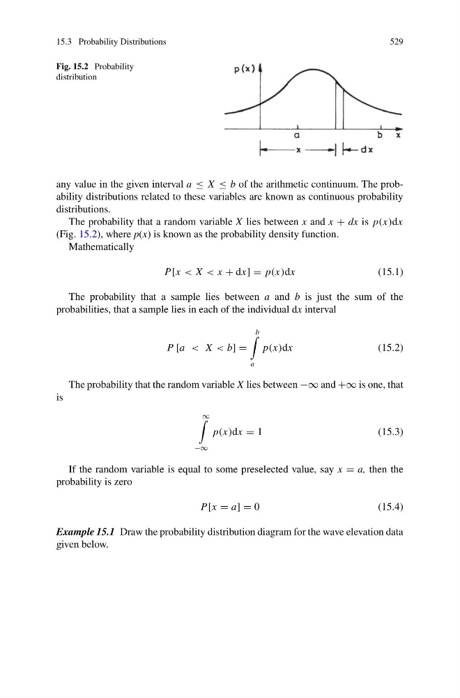
Fig. 15.2 Probability
distribution
any value in the given interval a ≤ X ≤ b of the arithmetic continuum. The probability distributions related to these variables are known as continuous probability
distributions.
The probability that a random variable X lies between x and x + dx is p(x)dx
(Fig. 15.2), where p(x) is known as the probability density function.
Mathematically
P[x < X < x + dx] = p(x)dx
(15.1)
The probability that a sample lies between a and b is just the sum of the
probabilities, that a sample lies in each of the individual dx interval
P [a < X < b] =
b
a
p(x)dx
(15.2)
The probability that the random variable X lies between −∞ and +∞ is one, that
is
∞
−∞
p(x)dx = 1
(15.3)
If the random variable is equal to some preselected value, say x = a, then the
probability is zero
P[x = a] = 0
(15.4)
Example 15.1 Draw the probability distribution diagram for the wave elevation data
given below.
529
Fig. 15.2 Probability
distribution
any value in the given interval a ≤ X ≤ b of the arithmetic continuum. The probability distributions related to these variables are known as continuous probability
distributions.
The probability that a random variable X lies between x and x + dx is p(x)dx
(Fig. 15.2), where p(x) is known as the probability density function.
Mathematically
P[x < X < x + dx] = p(x)dx
(15.1)
The probability that a sample lies between a and b is just the sum of the
probabilities, that a sample lies in each of the individual dx interval
P [a < X < b] =
b
a
p(x)dx
(15.2)
The probability that the random variable X lies between −∞ and +∞ is one, that
is
∞
−∞
p(x)dx = 1
(15.3)
If the random variable is equal to some preselected value, say x = a, then the
probability is zero
P[x = a] = 0
(15.4)
Example 15.1 Draw the probability distribution diagram for the wave elevation data
given below.