

520
14 Nonlinear Vibration
y(t) = y 0 (t) + hy 1 (t)
or
y (t) =
A
p
sin pt −
A
3 h
32 p 5 (3 sin pt − sin 3 pt)
(x)
p
2
= p
2
0 +
3
4
h
A
2
p 2
(y)
or
p 2 =
3
8
h A
2
+ p 0
1 +
3h A 2
2 p 0
(z)
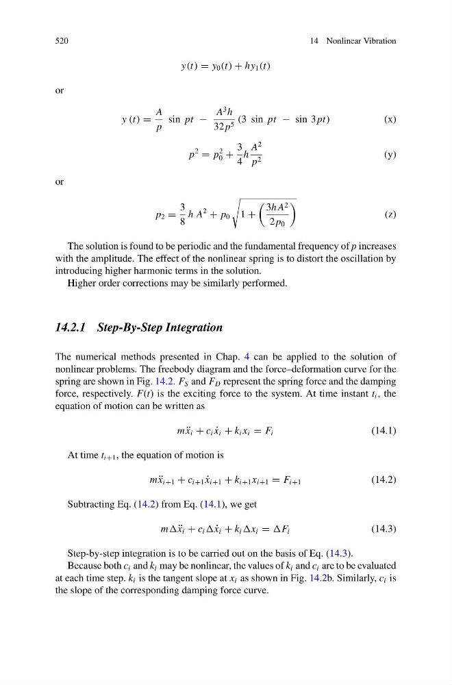
The solution is found to be periodic and the fundamental frequency of p increases
with the amplitude. The effect of the nonlinear spring is to distort the oscillation by
introducing higher harmonic terms in the solution.
Higher order corrections may be similarly performed.
14.2.1 Step-By-Step Integration
The numerical methods presented in Chap. 4 can be applied to the solution of
nonlinear problems. The freebody diagram and the force–deformation curve for the
spring are shown in Fig. 14.2. F S and F D represent the spring force and the damping
force, respectively. F(t) is the exciting force to the system. At time instant t i , the
equation of motion can be written as
m ¨
x i + c i ˙
x i + k i x i = F i
(14.1)
At time t i+1 , the equation of motion is
m ¨
x i+1 + c i+1 ˙
x i+1 + k i+1 x i+1 = F i+1
(14.2)
Subtracting Eq. (14.2) from Eq. (14.1), we get
m ¨
x i + c i ˙
x i + k i x i = F i
(14.3)
Step-by-step integration is to be carried out on the basis of Eq. (14.3).
Because both c i and k i may be nonlinear, the values of k i and c i are to be evaluated
at each time step. k i is the tangent slope at x i as shown in Fig. 14.2b. Similarly, c i is
the slope of the corresponding damping force curve.
14 Nonlinear Vibration
y(t) = y 0 (t) + hy 1 (t)
or
y (t) =
A
p
sin pt −
A
3 h
32 p 5 (3 sin pt − sin 3 pt)
(x)
p
2
= p
2
0 +
3
4
h
A
2
p 2
(y)
or
p 2 =
3
8
h A
2
+ p 0
1 +
3h A 2
2 p 0
(z)
The solution is found to be periodic and the fundamental frequency of p increases
with the amplitude. The effect of the nonlinear spring is to distort the oscillation by
introducing higher harmonic terms in the solution.
Higher order corrections may be similarly performed.
14.2.1 Step-By-Step Integration
The numerical methods presented in Chap. 4 can be applied to the solution of
nonlinear problems. The freebody diagram and the force–deformation curve for the
spring are shown in Fig. 14.2. F S and F D represent the spring force and the damping
force, respectively. F(t) is the exciting force to the system. At time instant t i , the
equation of motion can be written as
m ¨
x i + c i ˙
x i + k i x i = F i
(14.1)
At time t i+1 , the equation of motion is
m ¨
x i+1 + c i+1 ˙
x i+1 + k i+1 x i+1 = F i+1
(14.2)
Subtracting Eq. (14.2) from Eq. (14.1), we get
m ¨
x i + c i ˙
x i + k i x i = F i
(14.3)
Step-by-step integration is to be carried out on the basis of Eq. (14.3).
Because both c i and k i may be nonlinear, the values of k i and c i are to be evaluated
at each time step. k i is the tangent slope at x i as shown in Fig. 14.2b. Similarly, c i is
the slope of the corresponding damping force curve.