

14.2 Perturbation Method
521
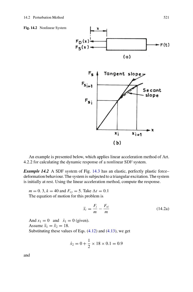
Fig. 14.2 Nonlinear System
An example is presented below, which applies linear acceleration method of Art.
4.2.2 for calculating the dynamic response of a nonlinear SDF system.
Example 14.2 A SDF system of Fig. 14.3 has an elastic, perfectly plastic force–
deformation behaviour. The system is subjected to a triangular excitation. The system
is initially at rest. Using the linear acceleration method, compute the response.
m = 0. 3, k = 40 and F sy = 5. Take t = 0.1
The equation of motion for this problem is
¨
x i =
F i
m
−
F si
m
(14.2a)
And x 1 = 0 and ˙
x 1 = 0 (given).
Assume ¨
x 1 = ¨
x 2 = 18.
Substituting these values of Eqs. (4.12) and (4.13), we get
˙
x 2 = 0 +
1
2
× 18 × 0.1 = 0.9
and
521
Fig. 14.2 Nonlinear System
An example is presented below, which applies linear acceleration method of Art.
4.2.2 for calculating the dynamic response of a nonlinear SDF system.
Example 14.2 A SDF system of Fig. 14.3 has an elastic, perfectly plastic force–
deformation behaviour. The system is subjected to a triangular excitation. The system
is initially at rest. Using the linear acceleration method, compute the response.
m = 0. 3, k = 40 and F sy = 5. Take t = 0.1
The equation of motion for this problem is
¨
x i =
F i
m
−
F si
m
(14.2a)
And x 1 = 0 and ˙
x 1 = 0 (given).
Assume ¨
x 1 = ¨
x 2 = 18.
Substituting these values of Eqs. (4.12) and (4.13), we get
˙
x 2 = 0 +
1
2
× 18 × 0.1 = 0.9
and