

506
13 Finite Difference Method for the Vibration Analysis …
are other possibilities of the amended scheme. The reader may check the amended
splines by substituting φ
i s from Eq. (13.43).
13.7.2 Displacement Functions
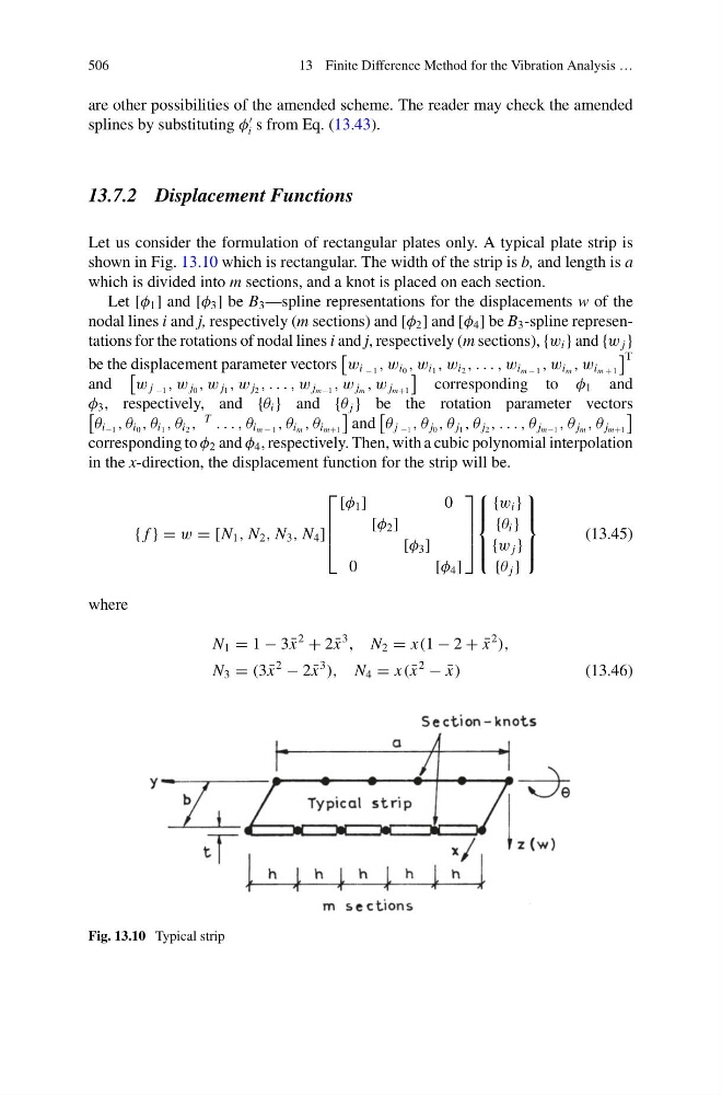
Let us consider the formulation of rectangular plates only. A typical plate strip is
shown in Fig. 13.10 which is rectangular. The width of the strip is b, and length is a
which is divided into m sections, and a knot is placed on each section.
Let [φ 1 ] and [φ 3 ] be B 3 —spline representations for the displacements w of the
nodal lines i and j, respectively (m sections) and [φ 2 ] and [φ 4 ] be B 3 -spline representations for the rotations of nodal lines i and j, respectively (m sections), {w i } and {w j }
be the displacement parameter vectors
w i − 1 , w i 0 , w i 1 , w i 2 , . . . , w i m − 1 , w i m , w i m + 1
T
and
w j −1 , w j 0 , w j 1 , w j 2 , . . . , w j m−1 , w j m , w j m+1
corresponding to φ 1 and
φ 3 , respectively, and {θ i } and {θ j } be the rotation parameter vectors
θ i −1 , θ i 0 , θ i 1 , θ i 2 ,
T
. . . , θ i m − 1 , θ i m , θ i m+1
and
θ j −1 , θ j 0 , θ j 1 , θ j 2 , . . . , θ j m−1 , θ j m , θ j m+1
corresponding to φ 2 and φ 4 , respectively. Then, with a cubic polynomial interpolation
in the x-direction, the displacement function for the strip will be.
{ f } = w = [N 1 , N 2 , N 3 , N 4 ]
⎡
⎢
⎢
⎣
[φ 1 ]
0
[φ 2 ]
[φ 3 ]
0
[φ 4 ]
⎤
⎥
⎥
⎦
⎧
⎪ ⎪ ⎨
⎪ ⎪ ⎩
{w i }
{θ i }
{w j }
{θ j }
⎫
⎪ ⎪ ⎬
⎪ ⎪ ⎭
(13.45)
where
N 1 = 1 − 3 ¯
x
2
+ 2 ¯
x
3
, N 2 = x(1 − 2 + ¯
x
2
),
N 3 = (3 ¯
x
2
− 2 ¯
x
3
), N 4 = x( ¯
x
2
− ¯
x)
(13.46)
Fig. 13.10 Typical strip
13 Finite Difference Method for the Vibration Analysis …
are other possibilities of the amended scheme. The reader may check the amended
splines by substituting φ
i s from Eq. (13.43).
13.7.2 Displacement Functions
Let us consider the formulation of rectangular plates only. A typical plate strip is
shown in Fig. 13.10 which is rectangular. The width of the strip is b, and length is a
which is divided into m sections, and a knot is placed on each section.
Let [φ 1 ] and [φ 3 ] be B 3 —spline representations for the displacements w of the
nodal lines i and j, respectively (m sections) and [φ 2 ] and [φ 4 ] be B 3 -spline representations for the rotations of nodal lines i and j, respectively (m sections), {w i } and {w j }
be the displacement parameter vectors
w i − 1 , w i 0 , w i 1 , w i 2 , . . . , w i m − 1 , w i m , w i m + 1
T
and
w j −1 , w j 0 , w j 1 , w j 2 , . . . , w j m−1 , w j m , w j m+1
corresponding to φ 1 and
φ 3 , respectively, and {θ i } and {θ j } be the rotation parameter vectors
θ i −1 , θ i 0 , θ i 1 , θ i 2 ,
T
. . . , θ i m − 1 , θ i m , θ i m+1
and
θ j −1 , θ j 0 , θ j 1 , θ j 2 , . . . , θ j m−1 , θ j m , θ j m+1
corresponding to φ 2 and φ 4 , respectively. Then, with a cubic polynomial interpolation
in the x-direction, the displacement function for the strip will be.
{ f } = w = [N 1 , N 2 , N 3 , N 4 ]
⎡
⎢
⎢
⎣
[φ 1 ]
0
[φ 2 ]
[φ 3 ]
0
[φ 4 ]
⎤
⎥
⎥
⎦
⎧
⎪ ⎪ ⎨
⎪ ⎪ ⎩
{w i }
{θ i }
{w j }
{θ j }
⎫
⎪ ⎪ ⎬
⎪ ⎪ ⎭
(13.45)
where
N 1 = 1 − 3 ¯
x
2
+ 2 ¯
x
3
, N 2 = x(1 − 2 + ¯
x
2
),
N 3 = (3 ¯
x
2
− 2 ¯
x
3
), N 4 = x( ¯
x
2
− ¯
x)
(13.46)
Fig. 13.10 Typical strip