

13.7 Spline Finite Strip Method of Analysis of Plate Vibration
505
φ i = 1/6h 3
⎧
⎪ ⎪ ⎪ ⎪ ⎪ ⎪ ⎪ ⎪ ⎪ ⎨
⎪ ⎪ ⎪ ⎪ ⎪ ⎪ ⎪ ⎪ ⎪ ⎩
0,
x < x i−2
(x − x i−2 ) 3 ,
x i−2 ≤ x ≤ x i−1
h 3 + 3h 2 (x − x i−1 ) + 3h(x − x i−1 ) 2 − 3(x − x i−1 ) 3 , x i−1 ≤ x ≤ x i
h 3 + 3h 2 (x i+1 − x) + 3h(x i+1 − x) 2 − 3(x i+1 − x) 3 , x i ≤ x ≤ x i+1
(x i+2 − x) 3 ,
x i+1 ≤ x ≤ x i+2
0,
x i+2 < x
⎫
⎪ ⎪ ⎪ ⎪ ⎪ ⎪ ⎪ ⎪ ⎪ ⎬
⎪ ⎪ ⎪ ⎪ ⎪ ⎪ ⎪ ⎪ ⎪ ⎭
(13.43)
The use of B 3 —splines offers certain distinct advantages when compared with
the conventional finite element method and semi-analytical finite strip method.
(1) It is computationally more efficient than the finite element method.
When using B 3 spline displacement functions, continuity is ensured up to
second order (C 2 —continuity). However, to achieve the same continuity conditions for the conventional finite element, it is necessary to have three times as
many unknowns at the nodes.
(2) It is more flexible than the semi-analytical finite strip method in the boundary
conditions treatment.
Only several local spline around the boundary point need to be amended to fit any
specified boundary conditions.
The B 3 —spline represents [φ] and can be easily managed to adapt to various
prescribed boundary condition. Due to the localization of the B 3 —splines, only three
boundary local splines have to be amended, i.e.
[] = [φ −1 , φ 0 , φ 1 , φ 2 , φ 3 , φ 4 , . . . , φ m−3 , φ m−1 , φ m , φ m+1 ]
(13.44)
in which the φ
i s are the standard local splines and the φ
i s are the amended local
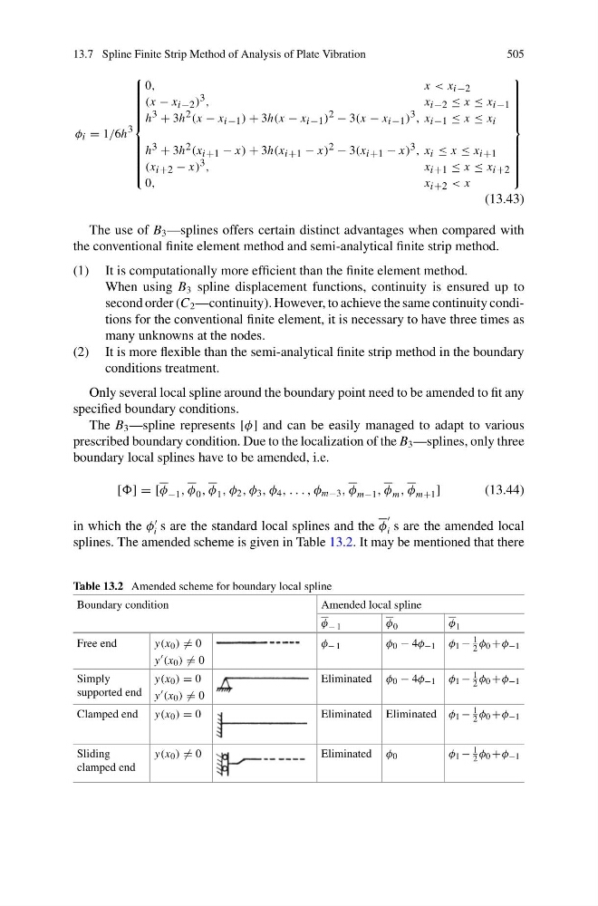
splines. The amended scheme is given in Table 13.2. It may be mentioned that there
Table 13.2 Amended scheme for boundary local spline
Boundary condition
Amended local spline
φ − 1
φ 0
φ 1
Free end
y(x 0 ) = 0
y (x 0 ) = 0
φ − 1
φ 0 − 4φ −1 φ 1 −
1
2 φ 0 +φ −1
Simply
supported end
y(x 0 ) = 0
y (x 0 ) = 0
Eliminated φ 0 − 4φ −1 φ 1 −
1
2 φ 0 +φ −1
Clamped end y(x 0 ) = 0
Eliminated Eliminated φ 1 −
1
2 φ 0 +φ −1
Sliding
clamped end
y(x 0 ) = 0
Eliminated φ 0
φ 1 −
1
2 φ 0 +φ −1
505
φ i = 1/6h 3
⎧
⎪ ⎪ ⎪ ⎪ ⎪ ⎪ ⎪ ⎪ ⎪ ⎨
⎪ ⎪ ⎪ ⎪ ⎪ ⎪ ⎪ ⎪ ⎪ ⎩
0,
x < x i−2
(x − x i−2 ) 3 ,
x i−2 ≤ x ≤ x i−1
h 3 + 3h 2 (x − x i−1 ) + 3h(x − x i−1 ) 2 − 3(x − x i−1 ) 3 , x i−1 ≤ x ≤ x i
h 3 + 3h 2 (x i+1 − x) + 3h(x i+1 − x) 2 − 3(x i+1 − x) 3 , x i ≤ x ≤ x i+1
(x i+2 − x) 3 ,
x i+1 ≤ x ≤ x i+2
0,
x i+2 < x
⎫
⎪ ⎪ ⎪ ⎪ ⎪ ⎪ ⎪ ⎪ ⎪ ⎬
⎪ ⎪ ⎪ ⎪ ⎪ ⎪ ⎪ ⎪ ⎪ ⎭
(13.43)
The use of B 3 —splines offers certain distinct advantages when compared with
the conventional finite element method and semi-analytical finite strip method.
(1) It is computationally more efficient than the finite element method.
When using B 3 spline displacement functions, continuity is ensured up to
second order (C 2 —continuity). However, to achieve the same continuity conditions for the conventional finite element, it is necessary to have three times as
many unknowns at the nodes.
(2) It is more flexible than the semi-analytical finite strip method in the boundary
conditions treatment.
Only several local spline around the boundary point need to be amended to fit any
specified boundary conditions.
The B 3 —spline represents [φ] and can be easily managed to adapt to various
prescribed boundary condition. Due to the localization of the B 3 —splines, only three
boundary local splines have to be amended, i.e.
[] = [φ −1 , φ 0 , φ 1 , φ 2 , φ 3 , φ 4 , . . . , φ m−3 , φ m−1 , φ m , φ m+1 ]
(13.44)
in which the φ
i s are the standard local splines and the φ
i s are the amended local
splines. The amended scheme is given in Table 13.2. It may be mentioned that there
Table 13.2 Amended scheme for boundary local spline
Boundary condition
Amended local spline
φ − 1
φ 0
φ 1
Free end
y(x 0 ) = 0
y (x 0 ) = 0
φ − 1
φ 0 − 4φ −1 φ 1 −
1
2 φ 0 +φ −1
Simply
supported end
y(x 0 ) = 0
y (x 0 ) = 0
Eliminated φ 0 − 4φ −1 φ 1 −
1
2 φ 0 +φ −1
Clamped end y(x 0 ) = 0
Eliminated Eliminated φ 1 −
1
2 φ 0 +φ −1
Sliding
clamped end
y(x 0 ) = 0
Eliminated φ 0
φ 1 −
1
2 φ 0 +φ −1