

13.5 Semi-analytic Finite Difference Method for Free Vibration …
499
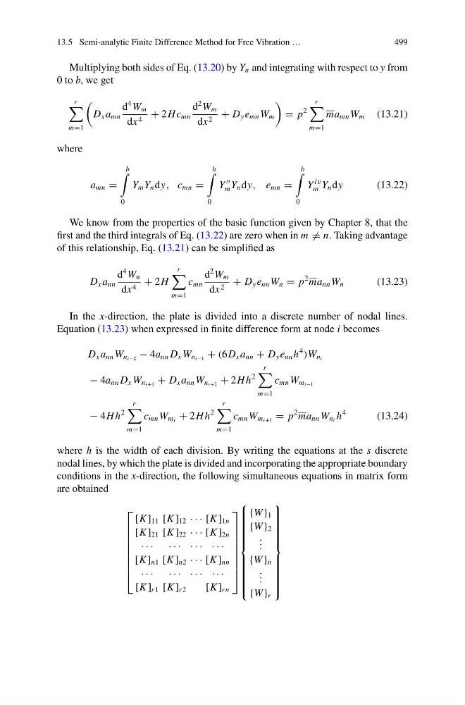
Multiplying both sides of Eq. (13.20) by Y n and integrating with respect to y from
0 to b, we get
r
m=1
D x a mn
d
4 W m
dx 4 + 2Hc mn
d
2 W m
dx 2 + D y e mn W m
= p
2
r
m=1
ma mn W m (13.21)
where
a mn =
b
0
Y m Y n dy, c mn =
b
0
Y
m Y n dy, e mn =
b
0
Y
iv
m Y n dy
(13.22)
We know from the properties of the basic function given by Chapter 8, that the
first and the third integrals of Eq. (13.22) are zero when in m = n. Taking advantage
of this relationship, Eq. (13.21) can be simplified as
D x a nn
d
4 W n
dx 4 + 2H
r
m=1
c mn
d
2 W m
dx 2 + D y e nn W n = p
2 ma nn W n
(13.23)
In the x-direction, the plate is divided into a discrete number of nodal lines.
Equation (13.23) when expressed in finite difference form at node i becomes
D x a nn W n i−2 − 4a nn D x W n i−1 + (6D x a nn + D y e nn h
4
)W n i
− 4a nn D x W n i+1 + D x a nn W n i+2 + 2H h
2
r
m=1
c mn W m i−1
− 4H h
2
r
m=1
c mn W m i + 2H h
2
r
m=1
c mn W m i+1 = p
2 ma nn W n i h
4
(13.24)
where h is the width of each division. By writing the equations at the s discrete
nodal lines, by which the plate is divided and incorporating the appropriate boundary
conditions in the x-direction, the following simultaneous equations in matrix form
are obtained
⎡
⎢
⎢
⎢
⎢
⎢
⎢
⎢
⎣
[K ] 11 [K ] 12 · · · [K ] 1n
[K ] 21 [K ] 22 · · · [K ] 2n
· · · · · · · · · · · ·
[K ] n1 [K ] n2 · · · [K ] nn
· · · · · · · · · · · ·
[K ] r 1 [K ] r 2
[K ] rn
⎤
⎥
⎥
⎥
⎥
⎥
⎥
⎥
⎦
⎧
⎪ ⎪ ⎪ ⎪ ⎪ ⎪ ⎪ ⎪ ⎪ ⎨
⎪ ⎪ ⎪ ⎪ ⎪ ⎪ ⎪ ⎪ ⎪ ⎩
{W } 1
{W } 2
. . .
{W } n
. . .
{W } r
⎫
⎪ ⎪ ⎪ ⎪ ⎪ ⎪ ⎪ ⎪ ⎪ ⎬
⎪ ⎪ ⎪ ⎪ ⎪ ⎪ ⎪ ⎪ ⎪ ⎭
499
Multiplying both sides of Eq. (13.20) by Y n and integrating with respect to y from
0 to b, we get
r
m=1
D x a mn
d
4 W m
dx 4 + 2Hc mn
d
2 W m
dx 2 + D y e mn W m
= p
2
r
m=1
ma mn W m (13.21)
where
a mn =
b
0
Y m Y n dy, c mn =
b
0
Y
m Y n dy, e mn =
b
0
Y
iv
m Y n dy
(13.22)
We know from the properties of the basic function given by Chapter 8, that the
first and the third integrals of Eq. (13.22) are zero when in m = n. Taking advantage
of this relationship, Eq. (13.21) can be simplified as
D x a nn
d
4 W n
dx 4 + 2H
r
m=1
c mn
d
2 W m
dx 2 + D y e nn W n = p
2 ma nn W n
(13.23)
In the x-direction, the plate is divided into a discrete number of nodal lines.
Equation (13.23) when expressed in finite difference form at node i becomes
D x a nn W n i−2 − 4a nn D x W n i−1 + (6D x a nn + D y e nn h
4
)W n i
− 4a nn D x W n i+1 + D x a nn W n i+2 + 2H h
2
r
m=1
c mn W m i−1
− 4H h
2
r
m=1
c mn W m i + 2H h
2
r
m=1
c mn W m i+1 = p
2 ma nn W n i h
4
(13.24)
where h is the width of each division. By writing the equations at the s discrete
nodal lines, by which the plate is divided and incorporating the appropriate boundary
conditions in the x-direction, the following simultaneous equations in matrix form
are obtained
⎡
⎢
⎢
⎢
⎢
⎢
⎢
⎢
⎣
[K ] 11 [K ] 12 · · · [K ] 1n
[K ] 21 [K ] 22 · · · [K ] 2n
· · · · · · · · · · · ·
[K ] n1 [K ] n2 · · · [K ] nn
· · · · · · · · · · · ·
[K ] r 1 [K ] r 2
[K ] rn
⎤
⎥
⎥
⎥
⎥
⎥
⎥
⎥
⎦
⎧
⎪ ⎪ ⎪ ⎪ ⎪ ⎪ ⎪ ⎪ ⎪ ⎨
⎪ ⎪ ⎪ ⎪ ⎪ ⎪ ⎪ ⎪ ⎪ ⎩
{W } 1
{W } 2
. . .
{W } n
. . .
{W } r
⎫
⎪ ⎪ ⎪ ⎪ ⎪ ⎪ ⎪ ⎪ ⎪ ⎬
⎪ ⎪ ⎪ ⎪ ⎪ ⎪ ⎪ ⎪ ⎪ ⎭