

12.9 Periodic Structures
487
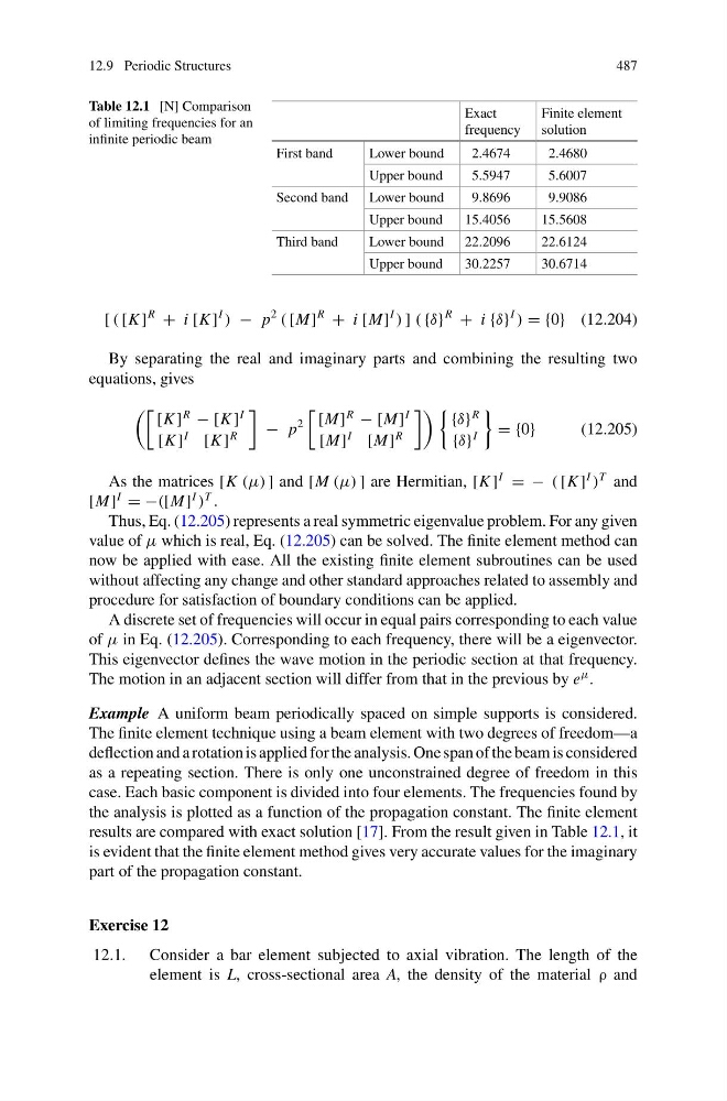
Table 12.1 [N] Comparison
of limiting frequencies for an
infinite periodic beam
Exact
frequency
Finite element
solution
First band
Lower bound
2.4674
2.4680
Upper bound
5.5947
5.6007
Second band Lower bound
9.8696
9.9086
Upper bound
15.4056
15.5608
Third band
Lower bound 22.2096
22.6124
Upper bound
30.2257
30.6714
[ ( [K ]
R
+ i [K ]
I
) − p
2
( [M]
R
+ i [M]
I
) ] ( {δ}
R
+ i {δ}
I
) = {0} (12.204)
By separating the real and imaginary parts and combining the resulting two
equations, gives
[K ]
R
− [K ]
I
[K ]
I
[K ]
R
− p
2
[M]
R
− [M]
I
[M]
I
[M]
R
{δ}
R
{δ}
I
= {0}
(12.205)
As the matrices [K (μ) ] and [M (μ) ] are Hermitian, [K ]
I
= − ( [K ]
I
)
T and
[M]
I
= −([M]
I
)
T .
Thus, Eq. (12.205) represents a real symmetric eigenvalue problem. For any given
value of μ which is real, Eq. (12.205) can be solved. The finite element method can
now be applied with ease. All the existing finite element subroutines can be used
without affecting any change and other standard approaches related to assembly and
procedure for satisfaction of boundary conditions can be applied.
A discrete set of frequencies will occur in equal pairs corresponding to each value
of μ in Eq. (12.205). Corresponding to each frequency, there will be a eigenvector.
This eigenvector defines the wave motion in the periodic section at that frequency.
The motion in an adjacent section will differ from that in the previous by e
μ .
Example A uniform beam periodically spaced on simple supports is considered.
The finite element technique using a beam element with two degrees of freedom—a
deflection and a rotation is applied for the analysis. One span of the beam is considered
as a repeating section. There is only one unconstrained degree of freedom in this
case. Each basic component is divided into four elements. The frequencies found by
the analysis is plotted as a function of the propagation constant. The finite element
results are compared with exact solution [17]. From the result given in Table 12.1, it
is evident that the finite element method gives very accurate values for the imaginary
part of the propagation constant.
Exercise 12
12.1. Consider a bar element subjected to axial vibration. The length of the
element is L, cross-sectional area A, the density of the material ρ and
487
Table 12.1 [N] Comparison
of limiting frequencies for an
infinite periodic beam
Exact
frequency
Finite element
solution
First band
Lower bound
2.4674
2.4680
Upper bound
5.5947
5.6007
Second band Lower bound
9.8696
9.9086
Upper bound
15.4056
15.5608
Third band
Lower bound 22.2096
22.6124
Upper bound
30.2257
30.6714
[ ( [K ]
R
+ i [K ]
I
) − p
2
( [M]
R
+ i [M]
I
) ] ( {δ}
R
+ i {δ}
I
) = {0} (12.204)
By separating the real and imaginary parts and combining the resulting two
equations, gives
[K ]
R
− [K ]
I
[K ]
I
[K ]
R
− p
2
[M]
R
− [M]
I
[M]
I
[M]
R
{δ}
R
{δ}
I
= {0}
(12.205)
As the matrices [K (μ) ] and [M (μ) ] are Hermitian, [K ]
I
= − ( [K ]
I
)
T and
[M]
I
= −([M]
I
)
T .
Thus, Eq. (12.205) represents a real symmetric eigenvalue problem. For any given
value of μ which is real, Eq. (12.205) can be solved. The finite element method can
now be applied with ease. All the existing finite element subroutines can be used
without affecting any change and other standard approaches related to assembly and
procedure for satisfaction of boundary conditions can be applied.
A discrete set of frequencies will occur in equal pairs corresponding to each value
of μ in Eq. (12.205). Corresponding to each frequency, there will be a eigenvector.
This eigenvector defines the wave motion in the periodic section at that frequency.
The motion in an adjacent section will differ from that in the previous by e
μ .
Example A uniform beam periodically spaced on simple supports is considered.
The finite element technique using a beam element with two degrees of freedom—a
deflection and a rotation is applied for the analysis. One span of the beam is considered
as a repeating section. There is only one unconstrained degree of freedom in this
case. Each basic component is divided into four elements. The frequencies found by
the analysis is plotted as a function of the propagation constant. The finite element
results are compared with exact solution [17]. From the result given in Table 12.1, it
is evident that the finite element method gives very accurate values for the imaginary
part of the propagation constant.
Exercise 12
12.1. Consider a bar element subjected to axial vibration. The length of the
element is L, cross-sectional area A, the density of the material ρ and