

486
12 Finite Element Method in Vibration Analysis
(12.199)
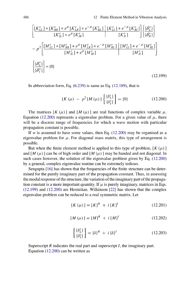
In abbreviation form, Eq. (6.239) is same as Eq. (12.189), that is
[K (μ) − p
2
[M (μ) ]
{δ
e
L }
{δ
e
I }
= {0}
(12.200)
The matrices [K (μ) ] and [M (μ) ] are real functions of complex variable μ.
Equation (12.200) represents a eigenvalue problem. For a given value of μ, there
will be a discrete range of frequencies for which a wave motion with particular
propagation constant is possible.
If w is assumed to have some values, then Eq. (12.200) may be organised as a
eigenvalue problem for μ. For diagonal mass matrix, this type of arrangement is
possible.
But when the finite element method is applied to this type of problem, [K (μ) ]
and [M (μ) ] can be of high order and [M (μ) ] may be banded and not diagonal. In
such cases however, the solution of the eigenvalue problem given by Eq. (12.200)
by a general, complex eigenvalue routine can be extremely tedious.
Sengupta [16] has shown that the frequencies of the finite structure can be determined for the purely imaginary part of the propagation constant. Thus, in assessing
the modal response of the structure, the variation of the imaginary part of the propagation constant is a more important quantity. If μ is purely imaginary, matrices in Eqs.
(12.199) and (12.200) are Hermitian. Wilkinson [22] has shown that the complex
eigenvalue problem can be reduced to a real symmetric matrix. Let
[K (μ) ] = [K ]
R
+ i [K ]
I
(12.201)
[M (μ) ] = [M]
R
+ i [M]
I
(12.202)
{δ
e
L }
{δ
e
I }
= {δ}
R
+ i {δ}
I
(12.203)
Superscript R indicates the real part and superscript I, the imaginary part.
Equation (12.200) can be written as
12 Finite Element Method in Vibration Analysis
(12.199)
In abbreviation form, Eq. (6.239) is same as Eq. (12.189), that is
[K (μ) − p
2
[M (μ) ]
{δ
e
L }
{δ
e
I }
= {0}
(12.200)
The matrices [K (μ) ] and [M (μ) ] are real functions of complex variable μ.
Equation (12.200) represents a eigenvalue problem. For a given value of μ, there
will be a discrete range of frequencies for which a wave motion with particular
propagation constant is possible.
If w is assumed to have some values, then Eq. (12.200) may be organised as a
eigenvalue problem for μ. For diagonal mass matrix, this type of arrangement is
possible.
But when the finite element method is applied to this type of problem, [K (μ) ]
and [M (μ) ] can be of high order and [M (μ) ] may be banded and not diagonal. In
such cases however, the solution of the eigenvalue problem given by Eq. (12.200)
by a general, complex eigenvalue routine can be extremely tedious.
Sengupta [16] has shown that the frequencies of the finite structure can be determined for the purely imaginary part of the propagation constant. Thus, in assessing
the modal response of the structure, the variation of the imaginary part of the propagation constant is a more important quantity. If μ is purely imaginary, matrices in Eqs.
(12.199) and (12.200) are Hermitian. Wilkinson [22] has shown that the complex
eigenvalue problem can be reduced to a real symmetric matrix. Let
[K (μ) ] = [K ]
R
+ i [K ]
I
(12.201)
[M (μ) ] = [M]
R
+ i [M]
I
(12.202)
{δ
e
L }
{δ
e
I }
= {δ}
R
+ i {δ}
I
(12.203)
Superscript R indicates the real part and superscript I, the imaginary part.
Equation (12.200) can be written as