

460
12 Finite Element Method in Vibration Analysis
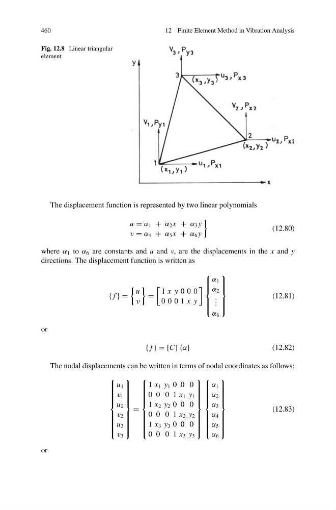
Fig. 12.8 Linear triangular
element
The displacement function is represented by two linear polynomials
u = α 1 + α 2 x + α 3 y
v = α 4 + α 5 x + α 6 y
(12.80)
where α 1 to α 6 are constants and u and v, are the displacements in the x and y
directions. The displacement function is written as
{ f } =
u
v
=
1 x y 0 0 0
0 0 0 1 x y
⎧
⎪ ⎪ ⎪ ⎨
⎪ ⎪ ⎪ ⎩
α 1
α 2
. . .
α 6
⎫
⎪ ⎪ ⎪ ⎬
⎪ ⎪ ⎪ ⎭
(12.81)
or
{ f } = [C] {α}
(12.82)
The nodal displacements can be written in terms of nodal coordinates as follows:
⎧
⎪ ⎪ ⎪ ⎪ ⎪ ⎪ ⎪ ⎨
⎪ ⎪ ⎪ ⎪ ⎪ ⎪ ⎪ ⎩
u 1
v 1
u 2
v 2
u 3
v 3
⎫
⎪ ⎪ ⎪ ⎪ ⎪ ⎪ ⎪ ⎬
⎪ ⎪ ⎪ ⎪ ⎪ ⎪ ⎪ ⎭
=
⎧
⎪ ⎪ ⎪ ⎪ ⎪ ⎪ ⎪ ⎨
⎪ ⎪ ⎪ ⎪ ⎪ ⎪ ⎪ ⎩
1 x 1 y 1 0 0 0
0 0 0 1 x 1 y 1
1 x 2 y 2 0 0 0
0 0 0 1 x 2 y 2
1 x 3 y 3 0 0 0
0 0 0 1 x 3 y 3
⎫
⎪ ⎪ ⎪ ⎪ ⎪ ⎪ ⎪ ⎬
⎪ ⎪ ⎪ ⎪ ⎪ ⎪ ⎪ ⎭
⎧
⎪ ⎪ ⎪ ⎪ ⎪ ⎪ ⎪ ⎨
⎪ ⎪ ⎪ ⎪ ⎪ ⎪ ⎪ ⎩
α 1
α 2
α 3
α 4
α 5
α 6
⎫
⎪ ⎪ ⎪ ⎪ ⎪ ⎪ ⎪ ⎬
⎪ ⎪ ⎪ ⎪ ⎪ ⎪ ⎪ ⎭
(12.83)
or
12 Finite Element Method in Vibration Analysis
Fig. 12.8 Linear triangular
element
The displacement function is represented by two linear polynomials
u = α 1 + α 2 x + α 3 y
v = α 4 + α 5 x + α 6 y
(12.80)
where α 1 to α 6 are constants and u and v, are the displacements in the x and y
directions. The displacement function is written as
{ f } =
u
v
=
1 x y 0 0 0
0 0 0 1 x y
⎧
⎪ ⎪ ⎪ ⎨
⎪ ⎪ ⎪ ⎩
α 1
α 2
. . .
α 6
⎫
⎪ ⎪ ⎪ ⎬
⎪ ⎪ ⎪ ⎭
(12.81)
or
{ f } = [C] {α}
(12.82)
The nodal displacements can be written in terms of nodal coordinates as follows:
⎧
⎪ ⎪ ⎪ ⎪ ⎪ ⎪ ⎪ ⎨
⎪ ⎪ ⎪ ⎪ ⎪ ⎪ ⎪ ⎩
u 1
v 1
u 2
v 2
u 3
v 3
⎫
⎪ ⎪ ⎪ ⎪ ⎪ ⎪ ⎪ ⎬
⎪ ⎪ ⎪ ⎪ ⎪ ⎪ ⎪ ⎭
=
⎧
⎪ ⎪ ⎪ ⎪ ⎪ ⎪ ⎪ ⎨
⎪ ⎪ ⎪ ⎪ ⎪ ⎪ ⎪ ⎩
1 x 1 y 1 0 0 0
0 0 0 1 x 1 y 1
1 x 2 y 2 0 0 0
0 0 0 1 x 2 y 2
1 x 3 y 3 0 0 0
0 0 0 1 x 3 y 3
⎫
⎪ ⎪ ⎪ ⎪ ⎪ ⎪ ⎪ ⎬
⎪ ⎪ ⎪ ⎪ ⎪ ⎪ ⎪ ⎭
⎧
⎪ ⎪ ⎪ ⎪ ⎪ ⎪ ⎪ ⎨
⎪ ⎪ ⎪ ⎪ ⎪ ⎪ ⎪ ⎩
α 1
α 2
α 3
α 4
α 5
α 6
⎫
⎪ ⎪ ⎪ ⎪ ⎪ ⎪ ⎪ ⎬
⎪ ⎪ ⎪ ⎪ ⎪ ⎪ ⎪ ⎭
(12.83)
or